CVMP 2008
Algorithms For Automatic And Robust Registration
Of 3D Head
Scans
urn:nbn:de:0009-6-26626
Abstract
Two methods for registering laser-scans of human heads and transforming them to a new semantically consistent topology defined by a user-provided template mesh are described. Both algorithms are stated within the Iterative Closest Point framework. The first method is based on finding landmark correspondences by iteratively registering the vicinity of a landmark with a re-weighted error function. Thin-plate spline interpolation is then used to deform the template mesh and finally the scan is resampled in the topology of the deformed template. The second algorithm employs a morphable shape model, which can be computed from a database of laser-scans using the first algorithm. It directly optimizes pose and shape of the morphable model. The use of the algorithm with PCA mixture models, where the shape is split up into regions each described by an individual subspace, is addressed. Mixture models require either blending or regularization strategies, both of which are described in detail. For both algorithms, strategies for filling in missing geometry for incomplete laser-scans are described. While an interpolation-based approach can be used to fill in small or smooth regions, the model-driven algorithm is capable of fitting a plausible complete head mesh to arbitrarily small geometry, which is known as "shape completion". The importance of regularization in the case of extreme shape completion is shown.
Keywords: nonrigid registration, ICP, geometry interpolation, morphable head models, shape completion, 3D face processing
Subjects: 3D-Scanner, Computational Geometry, Head
Laser scanners are a popular tool for acquiring detailed 3D models of human heads. However, the meshes generated by the scanners typically have a topology that reflects the operation of the scanner and is unsuitable for many applications. The data-set used in this work, for example, has a cylindrical grid topology with vertices of the form (ϕi, zi, ri) where ϕi are regularly spaced angles, zi are regularly spaced vertical offsets and ri are varying radii. In this paper, we describe two methods for semantically consistent registration and topology transfer of laser-scanned human heads that do not require manual intervention. The algorithms employ a user-provided template mesh which specifies the target topology. From arbitrary head scans they compute meshes with the following properties:
-
All generated meshes have the same topology, i.e. that of the reference mesh. Different heads only vary in vertex locations.
-
The mesh topology is semantically interpretable, i.e. topologically equivalent vertices in different heads have the same "meaning" such as tip of the nose, center of upper lip, etc.
The first algorithm proposed is purely geometric and computes the registration without prior knowledge. The second algorithm involves a semantic shape model of the human head, which is a variant of the popular morphable head model of Blanz and Vetter [ BV99 ]. While the model-driven algorithm is more robust than the geometric one, it presupposes a database of head meshes that are already registered in a common, semantically interpretable topology. Therefore, the geometric algorithm can be used to generate the database from which the model is computed. Both algorithms build on an error minimization approach computed in the well known Iterative Closest Points framework.
We also address the use of the registration algorithms with incomplete data, which is often an issue when laser-scanners or other surface reconstruction methods are used. For the geometric algorithm, we propose an interpolation method for filling in deficient areas that are either small or smooth. The model-driven algorithm can be used to fill in even huge missing parts with complicated geometry in a plausible fashion. In fact, with proper regularization, it is capable of performing "shape completion", i.e. computing plausible geometry that matches arbitrarily small pieces of given data.
The paper is structured as follows. In section 2 we give an overview of related work in the areas of ICP, morphable shape models and registration of head meshes. In section 3, we briefly recapitulate the algebra of first order ICP and introduce some notation. The geometric registration approach is described in section 4 and the model-driven scheme is treated in section 5.
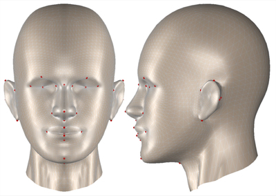
Figure 1. The reference mesh used for topology conversion with landmarks for the first algorithm stage.
Both algorithms use the Iterative Closest Points optimization scheme which was first introduced by Besl and MacKay [ BM92 ]. ICP is typically used to compute a rigid transform that aligns two or more partially overlapping meshes — e.g. laser-scans of a larger scene — such that the overlapping parts match as good as possible according to some error function. Common error functions are distances of closest points or point-to-plane distances (e.g. Chen and Medioni [ CM92 ]). The optimal transform depends on matching the right points in both meshes; to match the right points, however, the optimal transform must be known. Therefore, ICP assumes that the closest points match; the transform induced by these correspondences is computed and applied and the procedure is iterated. For a rigid transformation, ICP is guaranteed to converge to a minimum of the error function [ BM92 ]. However, this minimum may be local and thereby the meshes must be roughly aligned before ICP is invoked to find a good match.
There is a huge body of literature on ICP and numerous variants and optimizations have been proposed, aiming mostly at improving stability and speed of convergence. Rusinkiewicz and Levoy [ RL01 ] give an overview and, more recently, Mitra et al. [ MGPG04 ] introduced a general numeric optimization framework based on second order approximants which subsumes several previous approaches.
The ICP algorithm is neither limited to matching precisely overlapping meshes nor to the estimation of rigid transformations. In fact, any kind of transformation that is uniquely determined by a set of corresponding points can be estimated with ICP. However, as is the case for many optimization algorithms, the degrees of freedom of the transformation correlate with convergence: The more degrees of freedom there are, the more likely ICP is to converge to an undesired local minimum. Particularly relevant in the context of this work are non-rigid variants of ICP. These algorithms face the problem deforming the template in order to minimize the registration error while keeping its overall appearance. To this end, deformation is often controlled by a model that mimics the behavior of an elastic material. Examples of non-rigid ICP schemes are Haehnel et al. [ HTB03 ] who combine ICP optimization with a coarse to fine approach, or Amberg et al. [ ARV07 ] who minimize a nonrigid matching error function similar to that of Allen et al. ([ ACP03 ], see section 2.3) in a stepwise optimal fashion. Our model-driven algorithm (section 5) can be seen as a nonrigid ICP scheme with a data-driven deformation model; it was first published in [ SE09 ] where we compare it to other approaches and address its computational complexity.
"Morphable models" are orthogonal subspace models of 3D shape (and sometimes texture) of a certain object domain. In order to compute a morphable shape model, a database of meshes sharing the same semantically consistent topology is required. This allows to treat the geometry of a mesh with N vertices as a single measurement in a 3N-dimensional data-space. The morphable model is obtained by performing Principal Component Analysis (PCA) on the database in this space. By omitting eigenvectors with low eigenvalues a low-dimensional subspace covering the most dominant variations in the dataset is obtained. For complex shapes, a single linear subspace typically cannot cover sufficient variability. Therefore, the geometry is often split up into regions and each region is described by its own subspace model. Typically, regions overlap at their borders in order to obtain a smooth overall mesh in the end. Thereby, the morphable model becomes a PCA mixture model.
Morphable models have been used most successfully in the domain of the human head and face, where they were introduced as "morphable head models" by Blanz and Vetter [ BV99 ]. A wide number of applications in vision and graphics of faces can be driven or supported by morphable models, including, for example, face recognition [ AKV08, BV03 ], face tracking [ PF03, Rom05 ] and several varieties of 3D reconstruction, e.g. from uncalibrated video [ Fua00 ] or from stereo images [ ABF07 ]. While examples besides faces are rare, a morphable model of teeth is described in Blanz et al. [ BMVS04 ].
Head and face registration algorithms can roughly be divided into methods that exploit texture information and purely geometric approaches. On the side of geometric methods, some specialize exclusively on heads and faces while others try to solve the general problem of registering arbitrary surfaces by nonrigid transformations. The algorithms proposed in this paper belong to the class of head-specific purely geometric approaches. Several algorithms were introduced by the morphable model community since a database of registered meshes is required to compute a morphable model.
On the side of texture-based methods, Blanz and Vetter [ BV99, VB98 ] use an algorithm based on optical flow. Traditionally used to estimate 2D image deformation, optical flow is extended to use 2D texture as well as local 3D surface properties of the face in order to compute a matching deformation. However, the authors themselves [ BV99 ] as well as Paterson and Fitzgibbon [ PF03 ] report the method to be unreliable on "exotic" faces. Thus Paterson and Fitzgibbon [ PF03 ] manually annotate 30 landmark points in the texture and use radial basis function interpolation to compute a matching warp. 3D points are found by inverse-warping the texture coordinates associated with the 3D points.
Purely geometric head registration is used by Kähler et al. [ KHYS02 ] to animate facial expressions of laser-scanned heads with an anatomical animation model. Their method is based on iteratively subdividing a rough face mesh and aligning the new vertices to a reference model. The initial model for the subdivision is obtained from manually placed landmarks. Allen et al. [ ACP03 ] register full human body scans by using a generic nonlinear optimizer on an error function penalizing distances of closest points and dissimilarities between transforms of nearby points, thereby controlling the rigidity of the overall transformation. The approach requires some manually annotated landmarks to improve convergence. No landmarks are required by Anguelov et al. [ ASP05a ], who formulate the registration problem in the framework of a Markov random field. A variety of local and relational cost measures are incorporated in the field and the registration is computed by loopy belief propagation.
Geometric methods were also developed in the field of database retrieval and 3D face recognition. They typically aim at retrieving a stored prototype face from a database which is used to determine the identity of the scanned subject. To this end, Haar and Veltkamp [ tHV08 ] use curves originating from the nose in all directions. Nair and Cavallaro [ NC08 ] use ICP on incomplete faces in order to achieve invariance to facial expressions. These techniques, however, are designed to retrieve a model of the same person rather than registering multiple faces in a semantically valid way.
Issues of filling in incomplete data, which are addressed for both algorithms described in this work, are treated in several papers. Knothe et al. [ KRV06 ] use Local Feature Analysis, a localized variant of PCA, to fit a model to highly sparse data. Blanz et al. [ BMVS04 ] have a probabilistic approach for dealing with sparse fitting targets, where we propose a geometric regularization (sections 5.2 and 5.3). Anguelov et al. [ ASP05b ] perform shape completion on full body scans in arbitrary pose. Note that in this work, the issue of filling in smaller holes is dealt with in the context of the geometric algorithm, while shape completion and fitting to extremely sparse data is treated in the context of the model-driven approach.
Both algorithms treated in this paper are best described on the basis of the linearized ICP algorithm. In the following, we briefly recapitulate the algebra of this approach and introduce some notation.
Let rot(θ) denote a rotation matrix for a vector θ of
three Euler angles. Further, be t ∈
 3
a translation vector
and s an anisotropic scale factor. Be pi ∈
 3
a vertex of
the template mesh and qi ∈
 3
its corresponding point in
the target point cloud. Putting point-to-plane distances and
other optimizations aside, the ICP algorithm for estimating
rigid transformation and anisotropic scale minimizes the
following quadratic error function while simultaneously
establishing the correspondences between template meshand target point cloud:
 (1)
(1)
Here, N is the number of vertices in the template mesh.
A straightforward optimization strategy for ICP is to linearize this error functional around the parameter estimate (s,θ,t) of the last iteration and solve a linear system to find a small change in the parameters that decreases the error. Formally, this amounts to linearizing
 (2)
(2)
in (∆s, ∆θ , ∆t). To this end, rotation can be approximated as
 (3)
(3)
. where [p]x is the cross product matrix
 (4).
(4).
For a formal derivation, see, for example, [ WI95 ]. Expanding equation (2) and omitting higher order terms yields, after rearranging, the following linear system:
 (5)
(5)
For meshes of practical interest, this system is overdetermined and can be solved in a least squares sense, for example by SVD. The parameters are updated as follows:
 (6)
(6)
 (7)
(7)
 (8)
(8)
Note that rotation is maintained as a matrix and updated by multiplication rather than by adding up Euler angles in order to avoid gimbal lock. Finally, the updated transformation is applied and new point correspondences are established for the next iteration.
Since laser-scans are often incomplete, some vertices of the reference mesh may be assigned to overly far points in the cloud. These vertices have a large effect on the optimization due to the use of squared errors. Therefore, they should be treated as outliers by introducing a threshold on the distance between a template vertex and its target correspondence. Equations corresponding with outliers can be eliminated from the linear system in equation (5) by multiplying both sides with a diagonal binary matrix.
Our geometric registration algorithm comprises three steps: First, landmark points are found on the laser-scan mesh using the ICP scheme. Second, a nonlinear transform is computed to match the reference with the scan, using the landmark correspondences from step one as anchor points. Finally, the scan is resampled in the topology of the reference mesh and holes can be filled by interpolation.
In order to localize a landmark, the template mesh is repeatedly registered with the target point cloud. In every iteration, the ICP error function is re-weighted in order to concentrate the registration process on an increasingly smaller area around the landmark. The template mesh and the landmarks we use are shown in figure 1. The proposed localization strategy requires landmarks to have a non-flat, geometrically distinctive vicinity. Currently, landmark locations in the template are determined manually. However, slippage analysis introduced by Gelfand and Guibas [ GG04 ] could be an interesting approach to automatic search for suitable landmark locations.
For re-weighting, the ICP error of equation (1) is extended by a vertex specific factor wi, i = 1 ⋯ N which yields
 (9)
(9)
. This propagates to the linear system of equation (5) as a multiplication of the matrix with a diagonal weight matrix
 (10)
(10)
The role of the weights is to reduce the influence of the vertices distant from the landmark in an iterative manner. Generally, the weighting scheme should be a function ofthe form
 (11)
(11)
where pi is the vertex the weight of which is to be determined, L is the landmark that is currently processed, and α is a parameter that decreases with the iterations of the algorithm, controlling the size of the neighborhood that is to be considered in the ICP error term. Also, the weighting scheme must satisfy the constraints
 (12)
(12)
 (13)
(13)
Hence, by setting α = ∞ in the first iteration, unweighted ICP is performed.
There are numerous possibilities to implement this strategy. The most simple weighting scheme probably is the binary function
 (14)
(14)
where dist(pi,L) is a measure of distance from a vertex Pi to L. More complex weighting schemes replace the step function by a smooth falloff in L. Regarding the distance measure, there are again multiple possibilities. In our implementation, we use approximate geodesic distances computed with the fast marching algorithm of [ KS98 ]. Note that the distance measures can be precomputed and stored as long as the reference mesh stays constant.
In summary, the algorithm for finding all landmarks is the following:
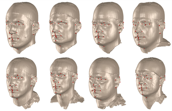
An illustration of the weighting function in the inner loop is shown in figure 3 for the upper lip landmark and the function of equation (14). Examples of automatically placed landmarks in different head scans are depicted in figure 2.
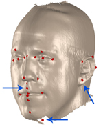
Depending on an individual head's geometry and on the quality of the laser-scan, the algorithm may converge to a bad localization of a landmark. Problem areas are the ears, where a good initial position of the template is required for good localization results, as well as the mouth where the geometry is not very pronounced for some individuals. A typical failure case in several landmarks is illustrated in figure 4. The algorithm also requires the scanned subjects to have the same facial expression as the template mesh. This is easiest to realize if both, subjects and template, display a neutral expression. Landmark localization quality is hard to evaluate numerically on our database since the low resolution of the laser-scans and lack of textures make a precise localization difficult for humans as well. However, the quality of the results is sufficient to build a morphable model that is capable of reproducing the facial characteristics of a wide range of individuals.
Figure 3. Landmark registration with an increasingly smaller area of influence for the error function: Example sequence of the influence area for the upper lip landmark with a binary weighting function.

Figure 4. Failure case of landmark registration: Ear, mouth and missing parts in the scan may lead to misregistration.
In the second step of the geometric algorithm, the template mesh is matched with the laser-scan point cloud in a global, nonlinear fashion using the established landmark correspondences. Denoting the landmarks in the template mesh by pi, i = 1 ⋯ K and their point cloud correspondences by qi , we seek a transformation Φ(⋅) such that Φ(pi) for all i and such that the points between the landmarks are interpolated in a natural fashion. This is nicely realized by the Thin Plate Spline formalism [ Boo89 ], which yields a transformation minimizing a physically interpretable bending energy. Similar non-linear deformation models have been used successfully in face processing before, e.g. in [ BKC08, BBA07 ].
From a Thin Plate Spline perspective we solve a three
dimensional scattered data interpolation problem from
 3
to
3
to
 3
. The known values are the displacement vectors
from the laser-scan landmark points to the reference mesh
landmarks,
 (15)
(15)
The unknowns to be interpolated are the displacement vectors of all non-landmark points in the reference mesh. Dealing with a three dimensional problem, the radial basis function to use for the spline is u(x) = |x| according to [ Boo89 ] and thus, with ui,j = || pi - pj||, we get a Thin Plate Spline matrix
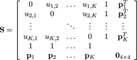 (16)
(16)
Hence the weight matrix for the mesh transform is
 (17)
(17)
and an arbitrary point v in the reference mesh transforms to
 (18)
(18)
with ui = || v - pi ||.
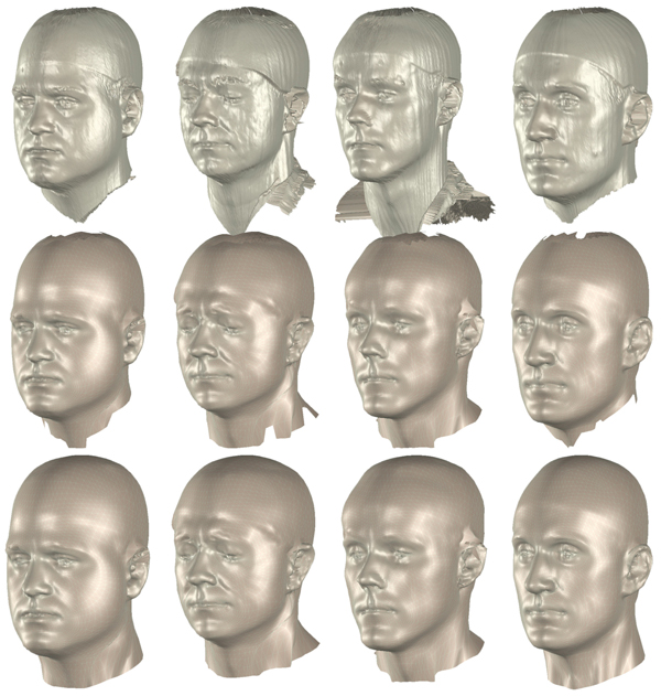
Figure 5. Results of the geometric registration algorithm. Top row: Original laser-scans. Middle row: Result after registration and topology transfer. Bottom row: Final result after hole-filling by offset interpolation.
The final step is to resample the laser-scan in the topology of the deformed reference mesh which now closely matches the scan. Therefore, for each vertex in the template mesh, its normal is computed and all intersections of the laser-scan with a line through the vertex in normal direction are determined. If there are multiple intersections, the one closest to the vertex is used. Moreover, there is a threshold on the distance between the vertex and the scan in order to exclude deficient matches at the scan's border. The chosen intersection point is taken as the correspondence to the template mesh vertex.
To speed up the computation of the ray-mesh-intersection, the laser-scan mesh is represented as an axis aligned bounding box tree and the fast ray box intersection of Williams et al. [ WBMS05 ] is used. Note that due to the size of a typical scan it is not feasible to build the tree down to the level of individual triangles. In our implementation with around 80 000 points in a scan, there are 100 triangles per leaf that have to be tested for each ray.
Due to scanning errors, the resampled scans have
holes where no valid correspondence along the normal
was found. The interpolation scheme described in
section 4.2 can be used to fill these holes as long as the
missing geometry is smooth and not too complex; a
model-based approach capable of filling in more complex
geometry is described in section 5.3. Again, we can
formulate the task as a scattered data interpolation
problem from
 3
to
3
to
 3
. Denote by hi
the vertices in the
template mesh that lack correspondence in the scan
(i.e. the vertices that make up the "hole"). Denote
by pj
vertices "surrounding the hole" that do have
correspondences qj
in the scan. The known values are the
displacements at the surrounding vectors dj = pj - qj
.
To be interpolated are the displacements
 at the vertices
lacking a reference. These can be computed with the
Thin Plate Spline formalism described above. Finally,
the correspondence of each "hole vertex" hi
is set to hi+
 .
.
Final results of the registration algorithm before and after hole filling are shown in figure 5.
The model-driven algorithm is based on a morphable model of head shape, which was computed as described in section 2.2. The database required to build the model was generated with the geometric registration algorithm reported above. For more details on the model-driven algorithm, including comparisons to other registration methods and issues of time complexity, see [ SE09 ].
In the following, be M the morphable shape model matrix and μ the model's mean vector. Hence the geometry of every mesh that can be represented by the model can be written as
 (19)
(19)
 (20)
(20)
is a single vector of all vertex coordinates and the parameter vector m is the location of the mesh in the model's "shape space". Note that our morphable model is a PCA mixture model comprising of six subspace models for mutually overlapping regions. Therefore, the model matrix is not simply a matrix of principal components. Details on the construction of M for the mixture model are given in section 5.1.
To use the morphable model for laser-scan registration, we again start from the ICP error functional of equation (1) and substitute equation (19) for the template mesh vertices pi :
 (21)
(21)
Note that in the above equation Mi and μi refer to three-row blocks of M and μ that correspond with individual mesh vertices. Additional to the scale and rigid transform parameters, the error now also depends on the shape parameter vector m. The addition of the shape model propagates to the matrix of the linear system of equation (5) as follows:
 (22)
(22)
See [ SE09 ] for a more detailed derivation. In the ICP loop, the system is now also solved for a shape change ∆m. The shape is initialized by m ← 0 which boils down to the mean shape μ of the model according to equation (19).
Once the model's shape and pose are fitted to the laser-scan, there are two ways to proceed: Either, the scan can be resampled by establishing correspondences along the normals of the template vertices, as in the geometric algorithm (section 4.3). Alternatively, the fitted morphable model may itself be used as the registered version of the laser scan. In this case, the results are, of course, confined to the space of shapes the model can represent. Which strategy is best depends on the application: Resampling the scan is computationally more expensive and gives noisier results but it preserves idiosyncrasies of the scanned individual that may not be captured by the model.
Note that due to the shape parameters, there are significantly more degrees of freedom in the error function minimized by the model-driven method than in that minimized by rigid ICP. Therefore, the result of the model-driven algorithm is more sensitive to the initial alignment of template and target. Best results are achieved when template and target are pre-aligned with respect to pose and anisotropic scale by regular ICP.
For a simple morphable model with a single subspace, the model matrix M is simply the eigenvector matrix yielded by the PCA. If a PCA mixture model with multiple subspaces is used, M has to constructed from the region's individual eigenvector matrices. See figure 6 for an illustration of the regions used in this work.
Figure 6. Partition of the head into regions for the PCA mixture model. Each part is described by its own subspace model.
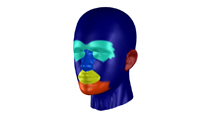
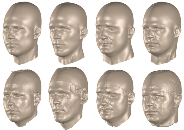
Figure 7. Results of the model-driven registration algorithm. Original laser-scans in the bottom row, fitted morphable model in the top row. Six region models and 15 principal components per region were used.
Assume the number of regions and hence the number of
subspaces used is K and denote each region's eigenvector
matrix by M(j),j = 1 ⋯ K. Further be
 1⋯
1⋯
 K
sets
of vertex indices such that i ∈
 j
if vertex pi
belongs to
region
 j
.
j
.
If the regions do not overlap, i.e.
 i ∩
i ∩
 j = ∅ for
i ≠ j, the matrix M has a block-diagonal structure:
 (23)
(23)
The results from this type of model, however, show harsh discontinuities between the regions since each region is optimized independently from the others. Therefore, the region models have to be coupled by introducing overlap at the region borders, i.e. vertices that belong to several regions. In consequence, the matrix M is no longer simply block diagonal.
If a vertex pi
belongs to region
 j its location is
determined by three consecutive rows of the region's
eigenvector matrix M(j)
, multiplied with the shape
parameters for that region. Denote these three rows of
M(j)
by Mi
(j)
and define
 (24)
(24)
where 0 is an all-zero matrix of appropriate size. Then, M can be defined block-wise as
 (25)
(25)
where αi (j) are block-weights satisfying
 (26)
(26)
Note that for a vertex pi that belongs just to one region, only one block Mi (j) is non-zero. As regions are typically defined to overlap only at their borders, the majority of vertices will be of this kind and M is fairly sparse.
The role of the block weights αi
(j)
is to normalize the
contributions of different region models for vertices that
belong to more than one region. The most simple block
weight is αi
(j)
 where Ri
is the number of regions the
vertex belongs to. If the area of overlap is deeper than just
one shared border vertex, more sophisticated weights
may be considered, giving more influence to some
regions than to others. In the following we give an
example of a weight that depends only on the mesh
topology.
Be a border edge an edge with only one incident
triangle and a border vertex a vertex that is incident to at
least one border edge. Denote by
 j
the set of border
vertices of region
 j
and by
 j
the index set of neighbors
of the vertex with index i. Now consider an arbitrary
vertex and define its "centricity" ci
(j)
with respect to
region
 j
recursively as
 (27)
(27)
Now the blending weight αi (j) can be defined as
 (28)
(28)
Equation (28) is equal to one for vertices that appear in only one part. For vertices appearing in multiple parts the weight is higher with respect to parts where the vertex is further away from the part border. The sum of blending weights of one vertex is always one, thus satisfying the constraint in equation (26).
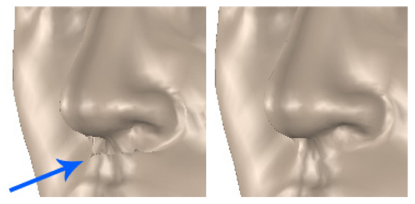
It is generally desirable to introduce as little overlap between the regions as possible: Large overlap increases the size of the linear system that has to be solved in every ICP iteration. Also, from a modeling point of view, every sub-model should ideally describe it's own part of the domain (here: the face) and interfere with other parts as little as possible. The downside to small overlap is the risk of discontinuities as shown in figure 8: The smaller the overlap, the more independent is the optimization of every region. As the optimization minimizes a sum of squared errors over all vertices in the region, two regions may yield significantly different locations for their shared vertices.
Figure 8. Effect of geometric regularization on a model with an overlap depth of one vertex. Left: A crease under the nose is clearly visible. Right: The same model fitted with geometric regularization.
This problem can be addressed — even for the smallest possible overlap of one shared line of vertices along the region border — by introducing a Tikhonov regularization term to the parameter estimation system. The aim of the regularization is to force shared vertices into the same position. Taking into account the block structure of M as defined in equation (25), we can write the location pi of a vertex given shape and pose parameters (s,θ,t,m) as
 (29)
(29)
Note that m(j)
is the part of the shape vector that
determines the shape of region
 j. Now assume that pi
is shared by exactly two regions
 S
and
S
and
 T
(i.e.
it is a vertex at the border between two regions).
Therefore, αi
(j) = 0 for all values of j except for {S,T}
and the summation in the above equation reduces
to αi
(S)Mi
(S)m(S)+αi
(T)Mi
(T)m(T)
. Clearly, the
two regions yield the same location for the vertex, if
T
(i.e.
it is a vertex at the border between two regions).
Therefore, αi
(j) = 0 for all values of j except for {S,T}
and the summation in the above equation reduces
to αi
(S)Mi
(S)m(S)+αi
(T)Mi
(T)m(T)
. Clearly, the
two regions yield the same location for the vertex, if
 (30)
(30)
This term can be expressed in matrix form and added to the linear system for every vertex that is a border vertex between two regions. For vertices shared by more than two regions, each unordered pair of regions yields one regularization term. In practice, these vertices can be ignored without harm.
In section 4.3 we sketched an interpolation algorithm that can be used to fill in holes in the laser-scans after registration with the geometric algorithm. The data-driven methodology, too, lends itself to a hole-filling — in fact the use of a model allows much more radical " filling in", up to the point of generating a plausible head that closely matches a very small piece of given geometry. This is sometimes referred to as shape completion in the literature.
Figure 9. Shape completion with the model-driven fitting algorithm. The fitting target is only a small piece of geometry (left). A plausible complete head (right) is fitted to the given data. Note that there is no given data for the ear region.
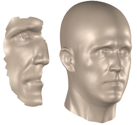
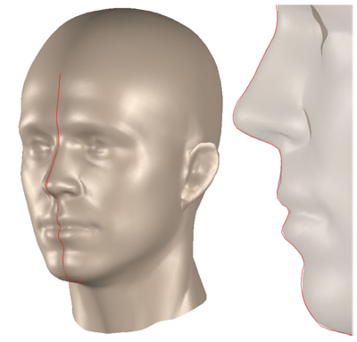
Figure 10. In this shape completion example, the target is only the red profile curve, which was extracted from a photo. The fitted head closely matches the target profile (right).
In order to cope with holes in the scan, outlier handling should be added to the optimization as described in section 3. Once the model is fitted to the scan, no additional filling or interpolation step is necessary: The shapes generated by the model are — by construction — always complete. Algebraically, this follows from the fact that the system of equation (22) loses rows when outliers occur but not columns. Therefore and regardless of the outliers, a complete shape parameter vector m is always computed. A full mesh is simply obtained by multiplying m with the the original shape matrix that contains all rows.
There is a caveat, however, if huge parts of the target geometry are missing, which is typical for the shape completion scenario. This can be seen by looking more closely at the effects of outlier removal on the matrix M. When a vertex with index i is classified as outlier due to the lack of a nearby target point, a three row block

corresponding to the outlier vertex is removed from M.
This is uncritical as long as there are sufficiently many
vertices left in the regions to which the removed vertex
belongs. What happens, however, if all information in a
region
 j is lost? It can be seen from the construction of
M in equation (25), that in this case all Mi
(j)
for
which αi
(j) ≠ 0 are lost and M contains a number of
zero-columns. In consequence, the elements of m that
determine the shape of the "unknown" region are
undetermined. If, however, geometric regularization is
used, there is still sufficient information in the Tikhonov
matrix to determine the shape parameters of region
 j
.
Geometrically, this is the information that whatever the
geometry of the region is, it must match the geometry of
its neighboring region in the shared vertices. Note that thisinformation also helps to prevent overfitting in the case of
very few inlier points. Figures 9 and 10 show some
extreme examples of shape completion. Note that in both
examples, the ears are completely undetermined by the
given data.
We described two robust methods for registering laser-scans of human heads and transforming them to a new semantically consistent topology defined by a user-provided template mesh. The first algorithm is based on finding landmark correspondences by iteratively registering the vicinity of a landmark with a re-weighted error function. Thin-plate spline interpolation is then used to deform the template mesh and finally the scan is resampled in the topology of the deformed template. The second algorithm directly optimizes pose and shape of a morphable shape model which can be computed using the results of the first algorithm. We outlined blending and regularization strategies for coping with PCA mixture models where the shape is split up into regions each described by an individual subspace. For both algorithms, we addressed strategies for filling in missing geometry for incomplete laser-scans. While the interpolation-based approach can fill in small or smooth regions, the model-driven strategy is capable of fitting a plausible complete head mesh to arbitrarily small geometry. We addressed the importance of regularization in the case of extreme shape completion.
Regarding the geometric algorithm, future research will concentrate on different re-weighting schemes in order to improve precision of automatic landmark placement, especially for difficult cases such as the ears and the corners of the mouth. For the model-driven method, an interesting open question is the choice of regions in the PCA mixture model. Currently, the regions are defined manually and based on an intuitive segmentation of the head into nose, mouth, eyes, etc. It would be interesting to investigate data-driven strategies that yield a segmentation as the result of an optimization process. The incorporation of classical ICP optimizations such as point-to-plane distances into both algorithms is another interesting direction of research.
[ABF07] Reconstructing High Quality Face-Surfaces using Model Based Stereo, Proc. International Conference on Computer Vision, pp. 1—8, 2007, isbn 978-1-4244-1630-1.
[ACP03] The Space Of Human Body Shapes: Reconstruction And Parameterization From Range Scans, Proc. of ACM SIGGRAPH, 2003, pp. 587—594, isbn 1-58113-709-5.
[AKV08] Expression Invariant 3D Face Recognition with a Morphable Model, 8th International Conference Automatic Face and Gesture Recognition, pp. 1—6, 2008, isbn 978-1-4244-2153-4.
[ARV07] Optimal Step Nonrigid ICP Algorithms for Surface Registration, Proc. Conference on Computer Vision and Pattern Recognition, 2007, pp. 1—8, isbn 1-4244-1180-7.
[ASP05a] The Correlated Correspondence Algorithm for Unsupervised Registration of Nonrigid Surfaces, Advances in neural information processing systems 17: proceedings of the 2004 conference, 2005, , pp. 33—40, isbn 9780262195348.
[ASP05b] SCAPE: Shape Completion and Animation of People, Proc. of ACM SIGGRAPH, pp. 408—416, 2005, issn 0730-0301.
[BBA07] Multi-Scale Capture of Facial Geometry and Motion, Proc. of ACM SIGGRAPH, 2007, Article no. 33, issn 0730-0301.
[BKC08] Facial Dynamics in Biometric Identification, Proc. British Machine Vision Conference, 2008.
[BM92] A Method for Registration of 3-D Shapes, IEEE Transactions on Pattern Analysis and Machine Intelligence, (1992), no. 2, 239—256, issn 0162-8828.
[BMVS04] A Statistical Method for Robust 3D Surface Reconstruction from Sparse Data, International Symposium on 3D Data Processing, Visualization and Transmission, 2004, pp. 293—300, isbn 0-7695-2223-8.
[Boo89] Principal Warps: Thin-Plate Splines and the Decomposition of Deformations, IEEE Transactions on Pattern Analysis and Machine Intelligence, (1989), no. 6, 567—585, issn 0162-8828.
[BV99] A Morphable Model for the Synthesis of 3D Faces, Proc. of ACM SIGGRAPH, 1999, 1063—1074, isbn 0-201-48560-5.
[BV03] Face Recognition Based on Fitting a 3D Morphable Model IEEE Transactions on Pattern Analysis and Machine Intelligence, (2003), no. 9, 1063—1074, issn 0162-8828.
[CM92] Object Modeling By Registration Of Multiple Range Images, Image and Vision Computing, (1992), no. 3, 145—155, issn 0262-8856.
[Fua00] Regularized Bundle-Adjustment to Model Heads from Image Sequences without Calibration Data, International Journal of Computer Vision, (2000), no. 2, 153—171, issn 0920-5691.
[GG04] Shape Segmentation Using Local Slippage Analysis, Eurographics Symposium on Gemetry Processing, 2004, pp. 214—223, isbn 3-905673-13-4.
[HTB03] An Extension of the ICP Algorithm for Modeling Nonrigid Objects with Mobile Robots, Proc. of the International Joint Conference on Artificial Intelligence, pp. 915—920, 2003.
[KHYS02] Head Shop: Generating Animated Head Models With Anatomical Structure, Proc. of ACM SIGGRAPH, 2002, pp. 55—63, isbn 1-58113-573-4.
[KRV06] Combining PCA and LFA for Surface Reconstruction from a Sparse Set of Control Points, International Conference Automatic Face and Gesture Recognition, pp. 637-644, 2006, isbn 0-7695-2503-2.
[KS98] Computing Geodesic Paths on Manifolds, Proc. of National Academy of Sciences, (1998), no. 15, 8431—8435, issn 0027-8424.
[MGPG04] Registration of Point Cloud Data from a Geometric Optimization Perspective, Eurographics Symposium on Geometry Processing, 2004, 22—31, isbn 3-905673-13-4.
[NC08] Matching 3D Faces with Partial Data, Proc. British Machine Vision Conference, 2008.
[PF03] 3D Head Tracking Using Non-Linear Optimization, British Machine Vision Conference 03, 609—618, 2003.
[RL01] Efficient Variants of the ICP Algorithm, Third International Conference on 3D Digital Imaging and Modeling, 2001, pp. 145—152, isbn 0-7695-0984-3.
[Rom05] Face Image Analysis using a Multiple Features Fitting Strategy, Universität Basel, 2005.
[SE09] Fast Nonrigid Mesh Registration with a Data-Driven Deformation Prior, ICCV Workshop on Non-Rigid Shape Analysis and Deformable Image Alignment, 2009.
[tHV08] A 3D Face Matching Framework, Proc. IEEE Shape Modeling International, 2008, pp. 103—110, isbn 978-1-4244-2260-9.
[VB98] Estimating coloured 3D face models from single images: An example based approach, Proc. European Computer on Computer Vision, 1998, pp. 499—513, isbn 3-540-64613-2.
[WI95] Iterative Estimation of Rotation and Translation using the Quaternion, Computer Science Department, Carnegie Mellon University, 1995, CMU-CS-95-215.
[WBM05] An Efficient and Robust Ray-Box Intersection Algorithm, International Conference on Computer Graphics and Interactive Techniques, 2005, Article no. 9.
Volltext 
-
 Volltext als PDF
(
Größe:
1.1 MB
)
Lizenz 
Jedermann darf dieses Werk unter den Bedingungen der Digital Peer Publishing Lizenz elektronisch übermitteln und zum Download bereitstellen. Der Lizenztext ist im Internet unter der Adresse http://www.dipp.nrw.de/lizenzen/dppl/dppl/DPPL_v2_de_06-2004.html abrufbar.
Empfohlene Zitierweise 
David C. Schneider, and Peter Eisert, Algorithms For Automatic And Robust Registration Of 3D Head Scans. JVRB - Journal of Virtual Reality and Broadcasting, 7(2010), no. 7. (urn:nbn:de:0009-6-26626)
Bitte geben Sie beim Zitieren dieses Artikels die exakte URL und das Datum Ihres letzten Besuchs bei dieser Online-Adresse an.
