Artikelaktionen
CVMP 2009
Sharpness Matching in Stereo Images
- Colin Doutre Department of Electrical and Computer Engineering, The University of British Columbia
-
Panos Nasiopoulos
 Department of Electrical and Computer Engineering, The University of British Columbia
Zusammenfassung
- eingereicht: 08.03.2010,
- akzeptiert: 01.02.2011,
- veröffentlicht: 25.04.2013
Keywords
- DOI: 10.20385/1860-2037/9.2012.4
- URN: urn:nbn:de:0009-6-32907
-
swd:
- 4478721-2
- 4615412-7
- 4690004-4
- 4279084-0
Sharpness Matching in Stereo Images
urn:nbn:de:0009-6-32907
Abstract
When stereo images are captured under less than ideal conditions, there may be inconsistencies between the two images in brightness, contrast, blurring, etc. When stereo matching is performed between the images, these variations can greatly reduce the quality of the resulting depth map. In this paper we propose a method for correcting sharpness variations in stereo image pairs which is performed as a pre-processing step to stereo matching. Our method is based on scaling the 2D discrete cosine transform (DCT) coefficients of both images so that the two images have the same amount of energy in each of a set of frequency bands. Experiments show that applying the proposed correction method can greatly improve the disparity map quality when one image in a stereo pair is more blurred than the other.
Keywords: stereo images, sharpness, blurring, depth estimation, discrete cosine transform (DCT)
Keywords: Stereo Images, Sharpness, Blurring, Depth Estimation, Discrete Cosine Transform (DCT)
SWD: Stereobild, Schärfe, Tiefenerkennung, Bildkontrast
Stereo matching is a classical problem in computer vision that has been extensively studied [ SS02 ]. It has many applications such as 3D scene reconstruction, image based rendering, and robot navigation. Most stereo matching research uses high quality datasets that have been captured under very carefully controlled conditions. However, capturing well-calibrated high quality images is not always possible, for example when cameras are mounted on a robot [ ML00 ], or simply due to a low cost camera setup being used. Capturing well calibrated stereo or multi-view video sequences is a challenging problem, and in fact many of the multiview sequences used by the Joint Video Team (JVT) standardization committee have noticeable inconsistencies between the videos captured with different cameras [ HOL07 ]. Inconsistencies between cameras can cause the images to differ in brightness, colour, sharpness, contrast, etc. These differences reduce the correlation between the images and make stereo matching more challenging, resulting in lower quality depth maps.
A number of techniques have been proposed to make stereo matching robust to radiometric differences between images (i.e., variations in brightness, contrast, vignetting). The images can be pre-filtered with a Laplacian of Gaussian kernel to remove changes in bias [ MKLT95 ]. Various matching costs have been proposed that are robust to variations in brightness such as normalized cross correlation [ Fua93 ] and mutual information [ KKZ03 ]. Another successful technique is to take the rank transform of the images [ ZW94 ], which replaces each pixel by the number of pixels in a local window that have a value lower than the current pixel. An evaluation of several matching techniques that are robust to radiometric differences is presented in [ HS07 ].
Much less work has addressed stereo matching when there are variations in sharpness/blurring between the images. Variations in image sharpness may result from a number of causes, such as the cameras being focused at different depths, variations in shutter speed, and camera shake causing motion blur.
In [ PH07 ], a stereo method is proposed using a matching cost based on heavily quantized DFT phase values. Their phase-based matching is invariant to convolution with a centrally symmetric point spread function (psf), and hence is robust to symmetric blurring. In [ WWH08 ] a method is proposed for performing stereo matching on images where a small portion of each image suffers from motion blur. A probabilistic framework is used, where each region can be classified as affected by motion blur or not. Different smoothness parameters in an energy minimization step are used for the pixels estimated as affected by motion blur. Note that neither [ PH07 ] nor [ WWH08 ] attempts to correct the blurring in the images (they do not modify the input images); instead, they attempt to make the matching more robust to blurring.
Although not a stereo matching technique, a method that does modify blurred multiview images is proposed in [ KLL07 ], for the purpose of coding multiview video when there is focus mismatch between cameras. In their method, first initial disparity vectors are calculated through block matching. Based on these vectors, the images are segmented into different depth levels. For each depth level, a filter is designed that will minimize the mean-squared error between the image being coded and a reference view being used for prediction. While this technique does modify the images to correct for sharpness variations, it only attempts to minimize the prediction error for a set of disparity estimates; it does not improve the disparity estimates themselves.
In this paper, we propose a fast method for correcting sharpness variations in stereo images. Unlike previous works [ PH07, WWH08 ], the method is applied as pre-processing before depth estimation. Therefore, it can be used together with any stereo method. Our method takes a stereo image pair as input, and modifies the more blurred image so that it matches the sharper image. Experimental results show that applying the proposed method can greatly improve the quality of the depth map when there are variable amounts of blur between the two images. The rest of this paper is organized as follows. The proposed method is described in section 2, experimental results are given in section 3 and conclusions are drawn in section 4.
When an image is captured by a camera, it may be degraded by a number of factors, including optical blur, motion blur, and sensor noise. Hence the captured image can be modeled as:
 (1)
(1)
where i(x,y) is the "true" or "ideal" image and h(x,y) is the point spread function (psf) of the capturing process. The '*' operator represents two dimensional convolution. The n(x,y) term is additive noise, which is usually assumed to be independent of the signal and normally distributed with some variance σn 2 . Throughout the paper, we will use the tilde '~' to denote an observed (and hence degraded) image. The psf, h(x,y), is usually a low-pass filter, which makes the observed image blurred (high frequency details are attenuated). In the case of stereo images, we have left and right images, iL and iR , for which the observed images can be modeled as in equation 1:
 (2)
(2)
If the same amount of blurring occurs in both images, i.e., hL and hR are the same, the images may lack detail but they will still be consistent. Therefore, stereo matching will still work reasonably well. We are interested in the case where different amounts of blurring occur in the images, so hL and hR are different. Our method attempts to make the more blurred image match the less blurred image by scaling the DCT coefficients of the images. The basis for our method is that un-blurred stereo images typically have very similar frequency content, so that the signal energy in a frequency band should closely match between the two images. Therefore, we scale the DCT coefficients in a set of frequency bands so that after scaling the image that originally had less energy in the band will have the same amount of energy as the other image. The resulting corrected images will match closely in sharpness, making stereo matching between the images more accurate. The steps of our method are described in detail in the following subsections
Typical rectified stereo image pairs have a large overlapping area between the two images. However, there is usually also a region on the left side of the left image and a region on the right side of the right image that are not visible in the other image (Fig. 1a). If these non-overlapping areas are removed, the assumption that the two images will have similar frequency content is stronger.
Figure 1. Removing non-overlapping edge regions. (a) Left and right original images with edge strips used in search shown in red and matching regions found through SAD search (equation 3 ) shown in blue. (b) Images cropped with non-overlapping regions removed.
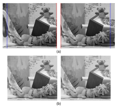
In order to identify the overlapping region between the two images, we consider two strips; one along the right edge of iL and one along the left edge of iR (see Figure 1a, regions highlighted in red). Strips five pixels wide are used in our experiments. We find matching strips in the other image using simple block based stereo matching. Using the sum of absolute differences (SAD) as a matching cost, two SAD values are calculated for each possible disparity d, one for the edge of iL and one for the edge of iR :
 (3)
(3)
The disparity value d that minimizes the sum SADL(d) + SADL(d) is chosen as the edge disparity D. Cropped versions of iL and iR are created by removing D pixels from the left of iL and D pixels from the right of iR (Figure 1b). These cropped images, which we will denote iLC and iRC, contain only the overlapping region of iLC and iRC.
In equation 3, we have used the standard sum of absolute differences as the matching cost. If there are variations in brightness between the images, a more robust cost should be used, such as normalized cross correlation or mean-removed absolute differences.
Noise can have a significant effect on blurred images, particularly in the frequency ranges where the signal energy is low due to blurring. We wish to remove the effect of noise when estimating the signal energy, which requires estimating the noise variance of each image.
We take the two dimensional DCT [
ANR74
] of the
cropped images, which we will denote as
 and
and
 . The indices u and v represent horizontal and
vertical frequencies, respectively. These DCT coefficients
are affected by the additive noise. We can obtain an
estimate for the noise standard deviation from the
median absolute value of the high frequency DCT
coefficients [
HSK04
]:
. The indices u and v represent horizontal and
vertical frequencies, respectively. These DCT coefficients
are affected by the additive noise. We can obtain an
estimate for the noise standard deviation from the
median absolute value of the high frequency DCT
coefficients [
HSK04
]:
 (4)
(4)
Values uT and vT are the thresholds for which DCT coefficients are classified as high frequency. We have used 20 less than the maximum values for u and v as the thresholds in our tests, meaning 400 coefficients used when calculating the median in equation 4. The reasoning behind equation 4 is that the high frequency coefficients are dominated by noise, with the signal energy concentrated in a small number of coefficients. The use of the median function makes the estimator robust to a few large coefficients which represent signal rather than noise. Using equation 4, we obtain estimates for the noise standard deviation in both images, σ N,L and σ N,R .
We wish to correct the full left and right images, without
the cropping described in section 2.1. Therefore, we
also need to take the DCT of the original images,
 and
and
 , so that those coefficients can be scaled.
This is in addition to taking the DCT of the cropped
images
and
, from which we will
calculate the scaling factors. The DCT coefficients of each
image have the same dimensions as the image in the
spatial domain. If the width and height of the original
images are W and H, the cropped images will have
dimensions (W - D) x H. In the DCT domain, the
dimensions of the coefficients will also be W x H for the
original images and (W - D) x H for the cropped
images.
, so that those coefficients can be scaled.
This is in addition to taking the DCT of the cropped
images
and
, from which we will
calculate the scaling factors. The DCT coefficients of each
image have the same dimensions as the image in the
spatial domain. If the width and height of the original
images are W and H, the cropped images will have
dimensions (W - D) x H. In the DCT domain, the
dimensions of the coefficients will also be W x H for the
original images and (W - D) x H for the cropped
images.
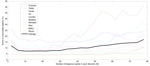
Figure 2. Division of DCT coefficients into M frequency bands in each direction, illustrated for M = 8.
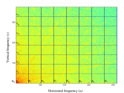
Our proposed method is based on the observation that stereo images typically have very similar amounts of energy in the same frequency ranges. Therefore, we divide the DCT coefficients of both the original and cropped images into a number of equally sized frequency bands, as illustrated in Figure 2.
Each frequency band consists of a set of (u,v) values such that ui ≤ u ≤ ui+1 and vj ≤ v ≤ vj+1 where ui is the starting index of band i in the horizontal direction and vj is the starting index of band j in the vertical direction (Figure 2). If we use M bands in both the horizontal and vertical directions, then the starting frequency index of each band in the original and cropped images are calculated as:
 (5)
(5)
where ui and vj are the indexes for the original images, and ui,c and vj,c are the indexes for the cropped images. Although ui and ui,c are different numbers, they correspond to the same spatial frequencies.
The number of frequency bands to use in each direction, M, is a parameter that must be decided. If more bands are used, the correction can potentially be more accurate. However, if too many bands are used, each band will contain little energy and therefore the estimate for the scaling factor will be less reliable. We evaluate the impact of the number of bands used experimentally in Section 3.1.
The DC coefficient for each image, IL(0,0) and IR(0,0), is treated as a special case, because the DC coefficient usually has much more energy than any of the AC coefficients, and has different statistical properties [ RG83 ]. Therefore, we treat the DC coefficient as a frequency band on its own (i.e. a band with only one coefficient). The size of the band is smaller for the DC coefficient, but otherwise the correction process is done the same as for the other bands.
Our assumption is that the true (un-blurred) images should have the same amount of energy in each frequency band. Therefore, we will scale the coefficients in each band so that the left and right images have the same amount of signal energy in each frequency band. The energy of each observed image in band ij can be computed as:
 (6)
(6)
We wish to remove the effect of noise from the energy calculated with 6. Let us define HI(u,v) as the DCT of the blurred signal h(x,y) * i(x,y), and define N(u,v) as the DCT of the noise. Since we are using an orthogonal DCT, N(u,v) is also normally distributed with zero mean and variance σn 2 . Given that the noise is independent of the signal and zero mean, we can calculate the expected value of the energy of the observed signal:
 (7)
(7)
Summing the above relation over all the DCT coefficients in a frequency band gives:
 (8)
(8)
where Enij(HI) is the energy of the blurred signal in frequency band ij and Cij is the number of coefficients in the band. The left hand side of equation 8 can be estimated with the observed signal energy calculated with equation 6. Therefore, we can estimate the blurred signal energy in the band with:
 (9)
(9)
In 9 we have clipped the estimated energy to be zero if the subtraction gives a negative result since the energy must be positive (by definition). Using 9 we estimate the signal energies Hnij(HIL) and Hnij(HIR). We wish to multiply the coefficients in the image with less energy by a gain factor (Gij) so that this image ends up having the same amount of signal energy as the other image. The scale factors to apply to each image in this band can be found as:
 (10)
(10)
 (11)
(11)
Note that either Gij,L or Gij,R will always be one. The gain factors calculated with 11 do not consider the effect of noise. If the signal energy is very low, the gain will be very high, and noise may be amplified excessively (this is a common issue in all image de-blurring methods [ GW02 ]). To prevent noise amplification from corrupting the recovered image, we multiply the gain by an attenuation factor, denoted A, which lowers the gain applied to the band based on the signal to noise ratio. Ideally, there would be no noise in the images, and we would be able to calculate the scaled DCT coefficients as . With noise, the scaled coefficients will G ∙ HI(u,v). With noise, the scaled coefficients will actually be G ∙ (HI(u,v) + N(u,v)). We choose the attenuation factor (A) to minimize the squared error between the ideal coefficients and the actual coefficients, i.e.,
 (12)
(12)
The value of A minimizes 12 is given by:
 (13)
(13)
where Enmin = min(En(HIL),En(HIR)) and σN,min 2 is the noise variance of the image that has less signal energy in the band. We provide a derivation for 13 in the appendix. Note that by attenuating the gain with equation 13, we are essentially using the classic Wiener filter [ Pra72, GW02 ] to limit the noise in the final images.
The scaling factors, G and A are calculated based on the DCT coefficients of the cropped images (because the assumption of equal signal energy in each frequency band will be stronger for the cropped images). So equations 6 through 13 are all applied only to the DCT coefficients of the cropped images. Once G and A are calculated for a frequency band ij, we scale the DCT coefficients of the original images:
 (14)
(14)
Note that we apply the same attenuation factor to the coefficients from both the left and right images. This ensures that the corrected images will have the same amount of signal energy in the band, at the expense of blurring the sharper image somewhat. However, unless the noise variance is very high in the blurred image, the sharper will not be affected much. Our method sharpens one image and smoothes the other, as the signal-to-noise ratio of the more blurred image limits how much we sharpening we can apply. An example showing the quality of the corrected images is shown in the results section (Figure 6).
After calculating all of the scaling factors, and applying equation 14 for every frequency band, we will have the complete DCT coefficients of the corrected images, IL,cor(u,v) and IR,cor(u,v). Then we simply take the inverse DCT to obtain the final corrected images in the spatial domain.
After applying our method a colour correction preprocessing method, for example histogram matching [ FBK08 ], could also be applied to reduce variations in brightness and colour between the images. Alternatively, a matching cost that is robust to variations in brightness could be used in subsequent stereo matching, such as those studied in [ HS07 ].
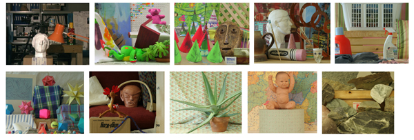
We test our proposed method on 10 stereo image pairs from the Middlebury stereo page [ SS11 ] that have ground truth disparities obtained through a structured light technique [ SS03 ]. Thumbnails of the test images are shown in Figure 3 . The 2005 and 2006 data sets from the Middlebury page (art, laundry, moebius, reindeer, aloe, baby1, rocks) all have seven views; we used the one-third size versions of views 1 and 3 as the left and right images in our tests.
Figure 3. Test images used in experiments (only left image of each pair is shown). In reading order: Tsukuba, teddy, cones, art, laundry, moebius, reindeer, aloe, baby1, and rocks.
Our sharpness correction method is a pre-processing step performed before stereo matching, and therefore it can be used together with any stereo method. We test our method together with two representative stereo algorithms; one simple window based matching method, and one global method that solves an energy minimization problem using Belief Propagation (BP) [ FH06 ].
Our window stereo method involves first performing block matching with a 9x9 window using sum of absolute differences (SAD) as the matching cost. A single disparity is chosen for each pixel that has the minimum SAD (winner take all). A left-right cross check is done [ Fua93 ] to invalidate occluded pixels and unreliable matches, and disparity segments smaller than 160 pixels are eliminated [ Hir03 ]. Invalid pixels are interpolated by propagating neighbouring background disparity values. Our window based method is similar to the window based method used for the comparative study in [ HS07 ]. The global belief propagation (BP) method solves a 2D energy minimization problem, taking into account the smoothness of the disparity field. We refer readers to [ FH06 ] for the details of the BP method.
Two kinds of blurring filters are tested. Out-of-focus blur, which is modeled with a disk filter of a given radius [ EL93 ], and linear motion blur, which is modelled as an average of samples along a straight line of a given length. We use the MATLAB commands fspecial('disk', ...) and fspecial('motion', ...) to generate the blurring filters.
The performance metric we use is the percentage of 'bad' pixels in the disparity map in the un-occluded regions of the image. A bad pixel is defined as one where the calculated disparity differs from the true disparity by more than one pixel. This is the most commonly used quality measure for disparity maps, and ithas been used in major studies such as [ SS02 ] and [ HS07 ].
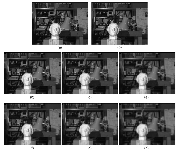
Figure 5. Demonstration of blurring filters used in our tests on the Tsukuba images (a) Original left image (b) Original right image, (c)-(g) Left image blurred with: (c) Out-of-focus blur, radius 1 (d) Out-of-focus blur, radius 2 (e) Out-of-focus blur, radius 3 (f) motion blur, length 2 (g) motion blur, length 3 (h) motion blur, length 4. The blurring filter is illustrated in the top left corner of each image.
In this section we evaluate how the performance of our method is affected by the number of frequency bands used in each direction (M), as described in section 2.4. We filtered the left image of each stereo pair with a disk filter of radius 2 (simulating an out of focus image) and added white Gaussian noise with variance 2. The right image was left unmodified. Then, we corrected the stereo pair using our algorithm a number of times, with the value of M ranging from 2 to 80. Finally, we ran the BP stereo matching method on the corrected images. The number of bad pixels versus the value of M is plotted in Figure 4 for the ten test image pairs, together with the average error across the ten image pairs.
From Figure 4, we can see that the amount of errors is generally higher when the number of bands is very low (2-6) or very high (50+). For all of the test images the number of errors is steady and near minimum when M is in the range 10 to 30. The average number of errors is minimized when M is 20.
Furthermore, choosing M = 20 gives very close to optimal results for all 10 test images.
We have done similar tests with other blur filters and different levels of blurring, and in all cases the results were similar to those shown in Figure 4 (i.e., the minimum was at or near M = 20, and the curves were flat in a large range around the minimum). Therefore we use M = 20 in the rest of our tests.
Here we compare the quality of depth maps obtained using our proposed method relative to performing stereo matching directly on the blurred images.
In each test, the right image was left unfiltered, while the left image was blurred with either a disk filter (simulating out-of-focus blur) or a linear motion blur filter at 45 degrees to the x-axis. We tested out-of-focus-blur with radii of 0, 1, 2 and 3 pixels and motion blur with lengths of 2, 3 and 4 pixels. A larger radius or length means the image is blurred more. A blur radius of zero means the image is not blurred at all, i.e., the filter is an impulse response and convolving it with the image leaves the image unaltered. White Gaussian noise with a variance of 2 was added to all of the blurred images (which is typical of the amount of noise found in the original images). Figure 5 shows the Tsukuba image blurred with all of the filters tested, to give the reader an idea of how severe the blurring is in different tests.
Table 1. Percentage of errors in disparity maps with Belief Propagation stereo method, out-of focus blurring
|
Radius |
Images |
Tsukuba |
Teddy |
Cones |
Art |
Laundry |
Moebius |
Reindeer |
Aloe |
Baby1 |
Rocks |
Average |
|
0 |
blurred |
2.0 |
14.8 |
9.7 |
6.8 |
13.2 |
7.9 |
5.9 |
2.8 |
1.6 |
3.8 |
6.8 |
|
|
corrected |
2.2 |
12.2 |
5.0 |
7.3 |
13.4 |
6.1 |
3.7 |
2.9 |
1.5 |
3.7 |
5.8 |
|
1 |
blurred |
3.3 |
16.6 |
12.9 |
8.9 |
13.0 |
8.0 |
8.0 |
3.9 |
1.7 |
4.2 |
8.1 |
|
|
corrected |
2.6 |
12.6 |
5.5 |
8.1 |
11.9 |
6.6 |
5.2 |
3.4 |
1.5 |
3.5 |
6.1 |
|
2 |
blurred |
6.4 |
28.1 |
28.4 |
13.2 |
18.6 |
12.4 |
15.3 |
8.4 |
6.2 |
7.0 |
14.4 |
|
|
corrected |
3.9 |
15.5 |
6.5 |
9.5 |
11.5 |
7.7 |
7.0 |
4.3 |
1.7 |
4.6 |
7.2 |
|
2 |
blurred |
11.0 |
39.6 |
55.3 |
26.8 |
33.1 |
26.5 |
24.5 |
32.1 |
25.8 |
16.3 |
29.1 |
|
|
corrected |
6.0 |
24.9 |
15.6 |
14.0 |
15.8 |
11.7 |
16.2 |
7.7 |
2.6 |
6.6 |
12.2 |
Table 2. >Percentage of errors in disparity maps with window stereo method, out-of focus blurring
|
Radius |
Images |
Tsukuba |
Teddy |
Cones |
Art |
Laundry |
Moebius |
Reindeer |
Aloe |
Baby1 |
Rocks |
Average |
|
0 |
blurred |
5.3 |
16.3 |
13.4 |
13.3 |
19.5 |
13.5 |
10.4 |
5.6 |
4.8 |
5.3 |
10.7 |
|
|
corrected |
5.4 |
14.4 |
8.4 |
15.0 |
19.5 |
12.2 |
7.4 |
5.8 |
4.9 |
6.7 |
10.0 |
|
1 |
blurred |
7.7 |
19.7 |
18.2 |
16.7 |
23.3 |
13.7 |
13.2 |
6.4 |
6.0 |
5.7 |
13.1 |
|
|
corrected |
8.0 |
17.4 |
8.4 |
16.3 |
17.8 |
12.9 |
11.9 |
5.9 |
5.1 |
5.1 |
10.9 |
|
2 |
blurred |
9.8 |
31.1 |
35.0 |
25.1 |
29.7 |
21.0 |
36.6 |
10.7 |
14.2 |
12.6 |
22.6 |
|
|
corrected |
8.8 |
23.9 |
10.1 |
19.4 |
18.7 |
15.4 |
26.4 |
7.0 |
6.7 |
8.4 |
14.5 |
|
3 |
blurred |
17.8 |
49.9 |
64.0 |
39.1 |
47.9 |
42.2 |
52.3 |
29.5 |
56.7 |
30.8 |
43.0 |
|
|
corrected |
10.6 |
44.3 |
31.4 |
27.2 |
33.7 |
24.1 |
42.6 |
12.6 |
13.4 |
13.2 |
25.3 |
Table 3. Percentage of errors in disparity maps with Belief Propagation stereo method, linear motion blur
|
Radius |
Images |
Tsukuba |
Teddy |
Cones |
Art |
Laundry |
Moebius |
Reindeer |
Aloe |
Baby1 |
Rocks |
Average |
|
2 |
blurred |
2.7 |
16.2 |
12.1 |
8.0 |
13.0 |
7.7 |
7.7 |
3.5 |
1.7 |
4.2 |
7.7 |
|
|
corrected |
2.6 |
12.5 |
5.3 |
8.1 |
12.2 |
5.5 |
5.4 |
3.0 |
1.4 |
3.6 |
6.0 |
|
3 |
blurred |
3.0 |
18.4 |
15.6 |
9.0 |
14.6 |
8.5 |
9.6 |
4.6 |
1.9 |
5.4 |
9.1 |
|
|
corrected |
2.6 |
13.1 |
5.9 |
8.1 |
10.8 |
6.0 |
5.6 |
3.6 |
1.6 |
4.3 |
6.2 |
|
4 |
blurred |
3.6 |
21.1 |
18.3 |
10.4 |
15.3 |
9.2 |
11.0 |
5.8 |
3.1 |
5.8 |
10.3 |
|
|
corrected |
3.0 |
14.5 |
6.4 |
8.5 |
10.9 |
7.1 |
6.4 |
4.1 |
1.6 |
4.1 |
6.7 |
Table 4. Percentage of errors in disparity maps with window stereo method, linear motion blur
|
Radius |
Images |
Tsukuba |
Teddy |
Cones |
Art |
Laundry |
Moebius |
Reindeer |
Aloe |
Baby1 |
Rocks |
Average |
|
2 |
blurred |
6.7 |
18.8 |
16.8 |
15.6 |
22.0 |
13.6 |
11.5 |
6.0 |
5.5 |
5.5 |
12.2 |
|
|
corrected |
6.7 |
16.3 |
8.5 |
16.0 |
19.3 |
12.5 |
9.2 |
5.9 |
4.7 |
5.0 |
10.4 |
|
3 |
blurred |
7.6 |
20.8 |
19.2 |
17.7 |
23.6 |
14.4 |
16.2 |
6.7 |
6.4 |
7.5 |
14.0 |
|
|
corrected |
6.5 |
17.2 |
8.9 |
17.0 |
17.2 |
13.0 |
15.3 |
6.1 |
5.1 |
5.8 |
11.2 |
|
4 |
blurred |
7.9 |
22.3 |
23.8 |
20.2 |
27.0 |
16.1 |
26.9 |
7.8 |
8.5 |
10.6 |
17.1 |
|
|
corrected |
7.2 |
19.8 |
10.3 |
17.4 |
20.2 |
13.5 |
21.7 |
6.7 |
5.5 |
7.4 |
13.0 |
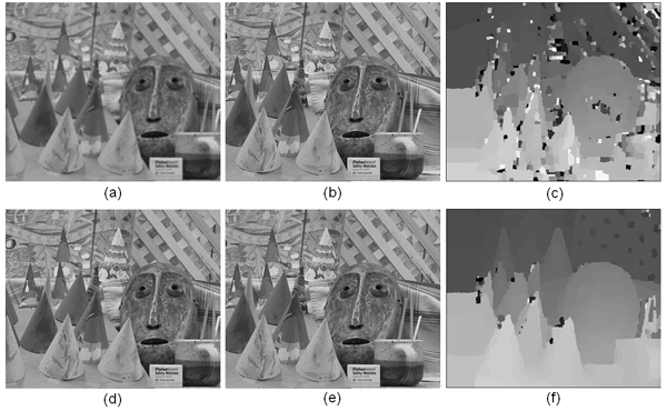
Figure 6. Example of cones image pair before and after correction. (a) Blurred left image (b) Original right image (c) Disparity map obtained from images a and b with Belief Propagation (d) Corrected left image (e) Corrected right image (f) Disparity map obtained from corrected images with Belief Propagation.
Tables 1 through 4 show the percentage of errors in the disparity maps obtained with different levels of blurring, with and without the proposed correction. The second column of each table (images) shows whether stereo matching was performed on either the blurred left image and original right image (the "blurred" case), or on the left-right pair obtained by applying our proposed method (the "corrected" case). Table 1 gives results for of-out-focus blur and the Belief Propagation stereo method, Table 2 for of-out-focus blur and the window stereo method, Table 3 for motion blur and the Belief Propagation stereo method, and Table 4 for motion blur and the window stereo method.
From Tables 1 through 4, we can see there is a substantial reduction in the number of errors in the disparity maps when the proposed correction is used, particularly when the amount of blurring in the left image is high. For the case of out-of-focus blur with a radius of 3 and the BP stereo method, the average number of errors is reduced from 10.7% to 10% using our proposed method. For all images, there is some improvement when the proposed correction is used if one image is blurred.
Even when neither image is blurred (the out-of-focus, zero radius case in Tables 1 and 2), there is some improvement on average when applying the proposed method. Using the Belief Propagation stereo method the average amount of errors is reduced from 6.8% to 5.8%, and for the window stereo method the average error is reduced from 10.7% to 10.0%, when neither image is blurred at all. One possible reason for this improvement is that through equation 13, noise is filtered from both images (the effect is similar to using a Weiner filter to remove noise [ Pra72 ]). Another possible reason is that the original images may have slightly different levels of sharpness that the proposed method can correct.
Comparing Tables 1 to Table 3, and Table 2 to Table 4, we can see that our correction method gives larger gains for out-of-focus blurring than for motion blur. This is because modifying the DCT coefficients can only correct for magnitude distortion, not phase distortion [ Mar94 ]. Since the out-of-focus blur filter is symmetric, it is zero-phase, and therefore introduces no phase distortion and can be accurately corrected for in the DCT domain. A linear motion blur filter is in general not symmetric, and hence introduces phase distortion. Modifying the DCT coefficients can correct the magnitude distortion caused by motion blur, but the corrected image will still suffer from phase distortion. Consequently, the proposed method provides some improvement for motion blur but not as much as it does for of-out-focus blur.
An example demonstrating the subjective visual quality of the corrected images and resulting disparity maps is shown in Figure 6. The blurred left image and original right image of the cones stereo pair is shown, along with the result of correcting the image pair with our method. The disparity maps obtained based on the blurred pair and corrected pair are also shown. Comparing (c) and (f) in Figure 6, we can see that the proposed method greatly reduces the errors in the disparity map, and produces more accurate depth edges. We can also see that the corrected images, (d) and (e), are perceptually closer in sharpness than the blurred images, (a) and (b). Therefore, the proposed method may also be useful in applications such as Free Viewpoint TV [ Tan06 ] and other multiview imaging scenarios, for making the subjective quality of different viewpoints more uniform.
Take the dimensions of the original left and right images as W x H. Removing the non-overlapping areas requires operations. We need to take four DCT's (of both original and cropped images). There are many fast algorithms for computing DCT's, which have complexity [ FJ05 ], where N is the number of pixels in the image, N = W ∙ H The number of operations required for the energy calculations and coefficient scaling is linear with the number of pixels, and therefore these steps have complexity. Finally two inverse DCT's must be performed to generate the corrected images in the spatial domain, which again have complexity. Overall, our proposed method has complexity, and the slowest steps are taking the DCT's and inverse DCT's of the images. Many fast algorithms, as well as software and hardware implementations, have been developed for performing the DCT and similar transforms [ FJ05 ]. We have implemented our proposed method in C code, and the running time for the Tsukuba images is 62 ms on an Intel Core 2 E4400 2 GHz processer under Windows XP. Therefore, the proposed method is fast enough to be used in real-time systems at reasonable frame rates.
In this paper we have proposed a pre-processing method for correcting sharpness variations in stereo image pairs. We modify the more blurred image to match the sharpness of the less blurred image as closely as possible, taking noise into account. The DCT coefficients of the images are divided into a number of frequency bands, and the coefficients are scaled so that the images have the same amount of signal energy in each band. Experimental results show that applying the proposed method before estimating disparity on a stereo image pair can significantly improve the accuracy of the disparity map compared to performing stereo matching directly on the blurred images.
Here we provide a detailed derivation for the value of the attenuation factor A given in equation 13. We wish to find the value of A which will minimize the difference between the desired scaled coefficients, G∙HI(u,v), and the noisy scaled coefficients G∙A(HI(u,v) + N(u,v)). The expected square error is:
 (15)
(15)
 (16)
(16)
Since the noise is zero mean and independent of the signal,E[N(u,v)] = 0 and the third and fifth terms in 16 are zero, so the equation reduces to:
 (17)
(17)
To find the minimum, we take the derivative with respect to A, and set it to zero:
 (18)
(18)
 (19)
(19)
The expected value E[N(u,v)2] is simply the noise variance. We can estimate the expected energy of an individual signal coefficient HI(u,v)2 , as the total signal energy in the band, calculated with equation (9), divided by the number of coefficients in the band (Cij).
 (20)
(20)
Rearranging gives the result of equation 13
[ANR74] Discrete Cosine Transform, IEEE Transactions on Computers, (1974), 1, issn 0018-9340.
[EL93] An investigation of methods for determining depth from focus, IEEE Trans. Pattern Analysis and Machine Intelligence, (1993), no. 2, 97—108 issn 0162-8828.
[FBK08] Histogram-based prefiltering for luminance and chrominance compensation of multiview video, IEEE Transactions on Circuits and Systems for Video Technology, (2008), no. 9, 1258—1267, issn 1051-8215.
[FH06] Efficient Belief Propagation for Early Vision, International Journal of Computer Vision, (2006), no. 1, 41—54, issn 0920-5691.
[FJ05] The Design and Implementation of FFTW3, Proceedings of the IEEE, (2005), no. 2, 216—231, issn 0018-9219.
[Fua93] A parallel stereo algorithm that produces dense depth maps and preserves image features, Machine Vision and Applications, (1993), no. 1, 35—49, issn 0932-8092.
[GW02] Digital Image Processing, 2nd Edition, Prentice Hall, 2002, isbn 978-0-130-94650-8.
[Hir03] Stereo Vision Based Mapping and Immediate Virtual Walkthroughs, De Montfort University, Leicester, UK, 2003.
[HOL07] Observations of Multi-view Test Sequences, Joint Video Team standard committee input document JVT-W084, Joint Video Team 23rd meeting, San Jose, USA , 2007.
[HS07] Evaluation of Cost Functions for Stereo Matching, Proc. IEEE Conference on Computer Vision and Pattern Recognition, 2007, pp. 1—8, isbn 1-4244-1180-7.
[HSK04] Reducing signal-bias from MAD estimated noise level for DCT speech enhancement, Signal Processing, (2004), no. 1, 151—162, issn 0165-1684.
[KKZ03] Visual correspondence using energy minimization and mutual information, Proc. IEEE Conference on Computer Vision, 2003, , pp. 1033—1040, isbn 0-7695-1950-4.
[KLL07] New Coding Tools for Illumination and Focus Mismatch Compensation in Multiview Video Coding, IEEE Trans. Circuits and Systems for Video Technology, (2007), no. 11, 1519—1535, issn 1051-8215.
[Mar94] Symmetric Convolution and the Discrete Sine and Cosine Transforms, IEEE Transactions on Signal Processing, (1994), no. 5, 1038—1051, issn 1053-587X.
[MKLT95] Obstacle detection for unmanned ground vehicles: a progress report, Proceedings of the Intelligent Vehicles '95 Symposium, 1995, pp. 66—71, isbn 0-7803-2983-X.
[ML00] Using real-time stereo vision for mobile robot navigation, Autonomous Robots, (2000), no. 2, 161—171, issn 0929-5593.
[PH07] Blur and Contrast Invariant Fast Stereo Matching, Proc. Advanced Concepts for Intelligent Vision Systems, Lecture Notes in Computer Science, 2007, , pp. 883—890, isbn 978-3-540-88457-6.
[Pra72] Generalized Wiener filtering computation techniques, IEEE Transactions on Computers, (1972), no. 7, 636—641, issn 0018-9340.
[RG83] Distributions of the two-dimensional DCT coefficients for images, IEEE Transactions on Communications, (1983), 835—839, issn 0090-6778.
[SS02] A Taxonomy and Evaluation of Dense Two-Frame Stereo Correspondence Algorithms, Int. Journal of Computer Vision, (2002), no. 1-3, 7—42, issn 0920-5691.
[SS03] High-accuracy stereo depth maps using structured light, Proc. IEEE Conference on Computer Vision and Pattern Recognition, 2003, , pp. 195—202, isbn 0-7695-1900-8.
[SS11] Middlebury stereo vision page, 2011, vision.middlebury.edu/stereo, last vistited March 2011.
[Tan06] Overview of Free Viewpoint Television, Signal Processing: Image Communication, (2006), no. 6, 454—461, issn 0923-5965.
[WWH08] Symmetric segment-based stereo matching of motion blurred images with illumination variations, Proc. International Conference on Pattern Recognition, 2008, pp. 1—4, isbn 978-1-4244-2174-9.
[ZW94] Non-parametric local transforms for computing visual correspondence, Proc. European Conference on Computer Vision, 1994, Lecture Notes in Computer Science Volume, , pp. 151—158, isbn 978-3-540-57957-1.
Volltext 
-
 Volltext als PDF
(
Größe:
3.6 MB
)
Volltext als PDF
(
Größe:
3.6 MB
)
Lizenz 
Jedermann darf dieses Werk unter den Bedingungen der Digital Peer Publishing Lizenz elektronisch übermitteln und zum Download bereitstellen. Der Lizenztext ist im Internet unter der Adresse http://www.dipp.nrw.de/lizenzen/dppl/dppl/DPPL_v2_de_06-2004.html abrufbar.
Empfohlene Zitierweise 
Colin Doutre, and Panos Nasiopoulos, Sharpness Matching in Stereo Images. JVRB - Journal of Virtual Reality and Broadcasting, 9(2012), no. 4. (urn:nbn:de:0009-6-32907)
Bitte geben Sie beim Zitieren dieses Artikels die exakte URL und das Datum Ihres letzten Besuchs bei dieser Online-Adresse an.
-
 News
News