CVMP 2009
A common problem in distributing digital images and movies is that of catering for varying image or film formats. For example a short sequence of a feature film may be shown on standard TV (768 x 576), HDTV (1920 x 1024), internet video (various), or even mobile phones (anything from 384 x 256 upwards). If shown for publicity reasons the producers will want this to be shown at the best quality possible. In effects houses which concentrate on advertising a significant proportion of time is spent just converting between the various digital formats on which the advertisement is to be shown. The problem arises because all digital images have to be sampled in order to be seen at all, but different kinds of display device have, of necessity, to show the images at differing resolutions.
Figure 1. Top to bottom: (a) Original digital photo (b) Rendered: flat-fill (c) Rendered: interpolated fill

Vector formats, historically associated with drawn images rather than with photographs, can provide a resolution-independent format but none of the existing fully automatic fill rules for vector formats work well on photographic images. This paper describes a new fill regime based on diffusion which results in images which are visually indistinguishable from their originals after conversion into and out of a vector representation. There are a number of systems and plug-ins available to turn images into vector form (e.g. Adobe Live Trace™ ) but they are all compromised by the absence of a good rule for determining varying colour values in a continuous field. Tools like Live Trace™ extract isochromic contours from sampled images but have to extract a sufficiently large number of contours to preserve the illusion of a smooth surface on a sampled display. This is because the usual rule for automatically filling between contours is to provide a constant colour (here called flat fill) in the viewable rasterised version of the image so the results can be thought of as providing a series of step changes in colour values rather than a continuous variation in those values. In Figure 1(b) we have used a flat fill regime on an image which was vectorised for a diffusion-based fill regime of the kind described later in this paper. The diffusion-based approach allows for the use of fewer contours without compromise to the appearance of smoother parts of the image and this has shown up a particular weakness of flat fill in the form of visible bands of colour changes (Mach bands). Indeed the usual application of such systems is to produce an artistic effect rather than a realistic outcome.
In this paper we show how to resolve this problem. As the contours can be thought of as a model of the image they need to be converted to a sampled image format in order to be seen on raster display devices. Thus a rendering process, entirely analogous to rendering processes used in 3D graphics, is required. The problem here is, if flat-fill is insufficient, how do we determine the intermediate pixel values between contours when rendering back to the sampled form? This problem and this paper's contribution to its solution are best illustrated in Figures 1(a)-(c) above. In Figure 1(b) the straightforward approach of flat fill has been taken. More explicitly each contour footprint, here defined as the image region uniquely enclosed by a contour, has been filled with a constant ' average' colour. In Figure 1(c) a diffusion-based interpolation technique (described in section 4) has been used instead. Each image was rendered from the same contour set. In Figure 1(b) the different outcomes are quite noticeable; flat fill shows Mach-banding artefacts which are wholly absent with the interpolated fill of Figure 1(c). As can be seen in Figure 1(c) the interpolating fill technique produces satisfactory results even though a quite simple rule has been used to determine which levels to use in the vector form.
A major problem in determining this vector form is that of determining how many contours to use. A naïve approach would be to use one contour for every unit of colour quantisation but this not only produces far more contours than are needed for a visually faithful reproduction of the image but also far more detail in defining each contour than is needed. If flat fill is used within contour boundaries the inefficient naïve approach is the only technique which will assure an artefact-free result. Techniques based on morphological principles (e.g. [ Ser82 ]) do this and, while we reference these techniques as part of the historical record, we would like to draw a distinction between the morphological approach and ours, notably in terms of the number of levels required for a visually satisfactory rendering. In such an approach all that would be needed for a visually faithful rendering would be to fill the contour with an 'average' colour quantised to be the border colour. In fact far fewer contours are needed in practice as we will show here.
Figure 2. Colour components and their contours: (a) Colour image, (b) Y-component, (c) U-component in greyscale, (d) V-component in greyscale, (e) Contourised Y for 2(b), (f) Contourised U for 2(c), (g) Contourised V for 2(d)
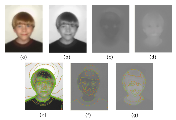
To illustrate the contours without too much visual confusion we chose the out-of-focus image Figure 2(a). Here the images have been rendered from contour sets representing the YUV components of a colour image. As can be seen in Figure 2(c),(d) and Figure 2(f),(g) there is very little detail in the U, V components so the size of the dataset is dominated by the Y-component. (This remains true even with a sharp, high-definition image.) The Y component (grey-scale) is held in levels-of-10 256 level quantisations, i.e. the colours 127, 127+10 etc. 127-10 etc. of which there are 25 altogether; while the U,V components, being more subtle in variation, are held in levels-of-5 (so 127, 127-5, 127-10 etc.) of which there are 49 altogether. This selection of contour levels has proved satisfactory for most of the images we have used here. We use Bézier chains to define contour borders, initially ignoring continuity between adjacent segments. The contours for the YUV components of Figure 2(a) are shown in Figure 2(e)(f)(g). The red contours are unsmoothed versions of the green ones. Smoothing is achieved by 'snapping' together end-point tangents if they fall within a certain threshold of being directionally opposite. This threshold value is one of several coefficients which can be modified to improve the image in one way or another.
This paper is structured as follows. The next section 2 covers previous work in this area, some of which reaches back to the earliest days of computer graphics. Section 3 discusses the main features of the vectorising codec we have used here, which has an encoder which works from a raster image to produce a vector image format and a decoder which renders the vector format back into a raster image. Section 4 discusses the decoding stage in more detail, and in particular the principles behind the diffusion-based interpolating fill process. We will see that this fill could be used just like any other area fill technique used in rendering vector format images, and on its own would give a drawing program (or Scalable Vector Graphics SVG[ DHH02 ] - interpreter) the ability to reconstruct contourised images to whatever degree of fidelity is required. Section 5 discusses some common image manipulation functions, including histogram equalisation, and here shows the consequences of producing truly rectangular histograms which are unachievable using sample-based techniques. Section 6 reviews where this work places vector image formats and section 7 will conclude the paper.
Vectorising (contourising) as applied to an array of
sample points is a technique whose origins go back to
geographical information systems
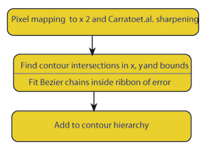
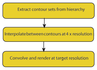
An image vectorising codec starts from a sampled image, typically one obtained from a digital camera, encodes it into an annotated contour set (derived as and collected into level sets) and subsequently decodes it back into a sampled image after whatever image transformation processes required are applied to it. A diagram of the main encoder stages used to produce the images in this paper is shown in Figure 3, and the corresponding decoder stages are shown in Figure 7.
We will now set out the principal features of our approach. In our codec individual contours are always represented by closed Bézier chains; contours clipped by the image border are completed by the shape of the border segment which falls within the contour footprint. This has certain implications for constructing the intermediate vector format and for the diffusion process involved in decoding (section 4.2). are found by first finding where they intersect lines between sample points derived from the original pixels. A key aspect of the input process is the explicit assumption that the pixel is contaminated by noise which can arise from any source, quantisation, sensor noise, even numerical inaccuracy, so is essentially of unknown origin. For example when considering the degree of accuracy to which the isosurface is modelled the strictest requirement we can safely make is that the isosurface model lies everywhere inside the error bounds of the pixels. error can be modelled in a number of ways, essentially either globally or locally. The accuracy of the value derived from the model is not critical although too crude a model could result in retaining image noise in the final result or a result which loses detail. While more accurate local approaches are covered in Patterson and Willis[ PW06 ] we should say that all the images in this paper were generated assuming a simple global noise value (∓ constant around each pixel value) without apparent loss of detail due to that assumption. If we are to attempt to preserve noise statistics in the final image, as suggested earlier, more accurate, local, methods will be needed. Error terms ε, however derived, can be converted into spatial errors δx , δy , in the x or y directions by applying the formulae:
 (1)
(1)
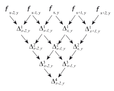
Here φ = φx,y is the piecewise continuous approximation of the 'true' isosurface. We now need to introduce some notation, as shown in Figure 4.
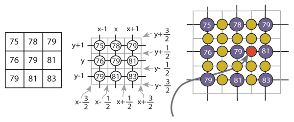
The first stage in the encoder is described as 'pixel mapping'. Here we double the image samples in each direction so that each set of 2 x 2 samples provided to the contour finder corresponds to a 'map' of the original pixel. However the new samples are all calculated by a non-linear process due to Carrato et al.[ SGS96 ] which emphasises edge detail, as more conventional interpolation (we use linear interpolation elsewhere for reasons which will be discussed shortly) does not introduce any new information.
The re-sizing step is in part intended to allow some distance between contours we take as adjacent although inevitably reconstructed edge values are often not identical with their original values (this is not noticeable to the naked eye) and the Carrato-sharpening is intended to defeat an ambiguity problem which arises in interpreting contour trajectories with the "marching squares" algorithm because of uncertainty over the centre sample in a pixel map. Carrato will bias the solution one way or another depending on surface topology and, although it would seem as though we have merely pushed the problem down to the next (second) level in fact linear interpolation is quite adequate for the second order case. (Surfaces tend to flatten out locally with more interpolants.) The scheme is illustrated in Figure 5(a)-(c).
Here Figure 5(a) shows what we mean by modelling
an image in terms of pixels, which may have many
interpretations[
Bli05
], but commonly (despite Smith[
Smi95
])
as little squares. For our purposes a more appropriate
model would be point samples addressed from the pixel
centre (Figure 5(b)). Figure 5(c) shows one of the
interpolated pixel values in red. Using the Carrato formula
this value would be calculated using the following
indices.

where

and

For the images in this paper we used the value p = 0.5. Similar equations prevail in the y-direction. The errors in the interpolated values are determined by subtracting the maximum and minimum interpolant values, using the limiting errors in the pixel values contributing to the result. For these differences, the index map for the error calculation is as follows.

the error εx,y is the (designated) error in Φx,y . The resultant error is then associated with the interpolated pixel which participates in all subsequent calculations indistinguishably from the originals.
The spatial errors in equation 1 are quoted in terms of continuous derivatives but once again we use first differences to generate the needed values, this time central differences, i.e. we use the formulae

where

(and corresponding formulae for the y direction). In the following discussion we will take ε = ±0.5, the quantisation error, which is the smallest value of ε can assume, but when encoding the image examples we have used here we essentially scaled ε by a constant amount chosen subjectively and intended to reflect our sense of how noisy the image was. Most digital images available to us have been through a process of JPEG encoding. It would be possible to trace through the decoding process to determine the per-pixel quantisation error which is typically image-dependent and spatially variable in that image, although we did not actually do this. For us the correct way of handling the effects of JPEG encoding is simply to use these quantisation errors as a lower bound for ε if other methods of estimating it are in play.
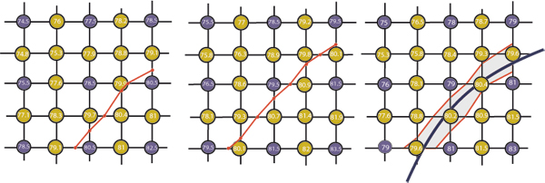
To show how a contour is determined we will use an example in which the error term is taken to be the quantisation error (±0.5). This is shown in Figure 6. If we determine the path of a contour in terms of its intersections with the borders of a box whose corners are decorated with sample values we can interpolate between sample values to get an 'exact' solution, thus allowing the 'exact' computation of the lower bound of the contour trajectory, Figure 6(a), and the upper bound, Figure 6(b). When these are transferred to the pixel tile with no error bound (ε = 0) they delimit the region we refer to as the ribbon of error within which any contour trajectory is equally valid. This is true for any realistic calculation for the pixel error. In fact we associate these errors with points on the contour line when fitting the Bézier chain but any fitting algorithm (e.g. the method outlined by Schneider[ Sch90 ] or by Vansichem et al.[ VWR01 ] has to take into account different values for that error around each sample point. One way to relax this condition is to multiply the derived error values with a constant and the consequence will be to reduce the number of segments in the chain and increase its smoothness.
It turns out that failing to take into account the presence of noise results in large numbers of Bézier segments in every contour as it twists and turns around single pixel-sized 'features' which are no more than noise-induced deviations from local correlation.
instead we account for noise adequately we get much smoother curves (with many fewer segments) whose smoothness has, up to a point, no perceptible effect on the resultant render. As indicated earlier the interpolation formula used is that for linear interpolation, that is by solving in the appropriate direction for the point where the linear interpolant along x or y is equal to the sought contour value, and then interpolating between the sample errors by the same amount. This is entirely equivalent to a process of solving for two isosurfaces, and is in fact safer, numerically. If we had used a local error measure then we could have determined which degree of interpolation was appropriate on a solution-by solution basis by finding which difference approximated to zero within the calculated error bounds for that difference[ PW06 ]. However past experiments with a pixel-level noise estimator have showed that for the majority of cases (approximately two-thirds in typical images) only linear interpolation could be justified and the rather basic assumptions about noise made here would not justify higher order interpolation anywhere. The resulting polyline approximation to the 'true' contour is simplified by finding the Bézier chain with the fewest segments which fit within the error ribbon the polyline approximation defines.
In an encoder the contour values can be determined by a blind strategy or an adaptive strategy. In this paper we have used a simple but (reasonably) effective blind strategy of pre-selecting the values to be found. As a consequence all the images in this paper are represented by the same choice of contour levels and all the contours are found at the same time by a single scan of the image from top to bottom. Here we examine each pixel to see which contours pass through a bounding box around its centre and then join up the contours by matching adjacent bounding box edges. This scan-based approach is only really possible with a blind strategy as an adaptive strategy will of necessity contain a stopping condition based on testing the need for the contour loop under consideration.
The outcome of the process is a hierarchy of contours (including contours R and S) defined in terms of the relation R encloses S defined as follows in terms of closed connected regions such as A . To define encloses(,) we start with the well-known inside test inside() where p inside A ⊃ WA(p) = s where WA(p) is the winding number for p in the closed region A and s is consistently +1 or -1 for every point p in the region. Now we need footprint() defined as:

and hence:

So AenclosesB is an ordering relation between individual closed contours in each level and determines all the contours B which are enclosed by A and by no other contour. Rendering the vector format consists of rules for drawing and filling these contours in order. The decoder, shown here as Figure 7, 'simply' applies the fill rule for the footprint of each pair of contours in the hierarchy as defined by the footprint of the enclosing contour subtracted from the footprint of all the contours it encloses directly. So although (here) contours are generated in levels (i.e. all the contours at a given level) they are ordered in terms of individual pairs of contours.
The principal issue in rendering is to use a process which mimics to some degree the fall-off in values of pixels from a higher level to an adjacent lower one (or vice-versa). The intention is to develop a simple diffusion-based fill algorithm between levels, as defined by level lines (isochromic contours). We will first develop the idea in Level Set terms and then show how to implement it without having to solve the differential equations which the invocation of level sets implies. The reason for doing this is that Level Set theory makes the issues clear in a direct and easily visualisable manner but the complexities of solving the equations led us to use known fast, scanline based methods to give us quick renders.
Figure 8. Contour creation (a) Dilation of ψ to include R, (b) Contraction of ψ inside S, (c) Reconciliation of R and S indices, (d) Pinching of isochromic contour by shape, (e) Effect of two interior contours on intermediates, (f) Effect of two interior contours on intermediates
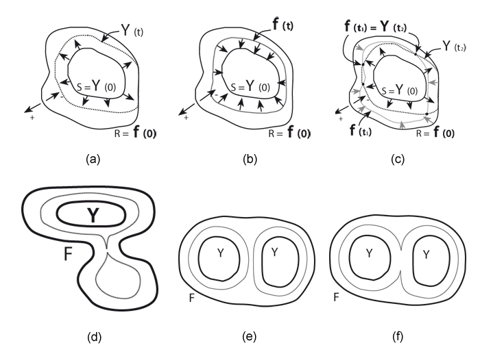
We derive the formulae in terms of a simple case (Figure 8) of a single outer contour with level value R surrounding a single inner contour level S, and then generalise. We want to arrange for the inner contour S = ψ(0) to first expand (in the terminology of Vincent[ Vin93 ]: 'to dilate') at a uniform (unit) speed until it wholly contains R (Figure 8(a)). At all times the level line for ψ(t) over the interval 0 ≤ t ≤ 1 gives the shape of the intermediate dilation at instant t which we note is wholly dependent on the shape of S and has no connection with the shape of R. If, at the same time, the corresponding level line for R is contracted ('eroded'[ Vin93 ], as in Figure 8(b) at uniform speed until it falls wholly within S then the level lines for intermediate erosion at time point t2 , say, will intersect the level lines for dilation in a range around another time point t1 . These time points t1 and t2 now correspond to the times taken to reach the nearest points on R and S respectively, so define linear distances within R - S (R with S removed from within it) which can be used to interpolate colours associated with R and S respectively at the points of intersection of these two curves. In fact we can go further and say that if we take any point p inside R - S then the time taken to reach it from R is the morphological distance from the boundary of R, and the time taken to reach it from S is the corresponding distance from S. So by using these distances as interpolants we get (within later caveats) the right intermediate colour for the point p.
Reviewing and extending what we have said so far, for any point inside the region R - S the shortest distances to the boundaries of R and S respectively determine the interpolation of the colours associated with the bounding levels R.S at that point. These interior colours will usually vary linearly from the values associated with one contour to the other, but this only happens if the geodesics running through the points in question are straight lines, i.e. the boundaries are not occluded from the point. In more complicated situations this approach generates interior colours which vary as though affected by surface tension, which is likely to fit what is actually found. This is shown further in Figure 8(d) where the intermediate contour or isochromic line is actually split into two and there is a local 'bubble' in the middle of the lower lobe of the outer contour. An analogous situation is shown in Figure 8(e) and (f), where there are two interior contours in the footprint of the outer contour. In Figure 8(e) the isochromic line has not yet joined up while it has done so in (f).
Taking the outwards direction as positive (as shown in Fig 9(a), the level set equation for the expansion (dilation) of ψ is:

 (2)
(2)
Here ψ(t) is the expansion of ψ(0) clipped by R = ψ(0).
The function dist() gives geodesic distances of points in R, R(a) say, from S using the value of t at the points at which ψ(t) = R(a). It is defined formally in the Appendix but may informally be thought of as the geodesic distance between two points, or a point and a boundary within an irregular, complete enclosure on a finite plane.
We can obtain the morphological distance fields for -R and +S by evaluating equation 2 and its matching partner for the erosion[ Vin93 ] of R, equation 3 as in Figure 3(b):

 (3)
(3)
This will give two Euclidean distances t1 , t2 , where ψ(t)1 = ψ(t)2 at zero or more points inside R - S (as in Figure 3(c)) so we can calculate the colour values C of those points from the colours CR, CS associated with level lines S and R respectively as:

We have used diffusion twice to give us morphological distances from each point in space in terms of the time to reach each of the two levels (here the speed of travel is unity so time = distance). When normalised by the sum of the distances this gives us an interpolation ratio between the two contour values which is linear for simple geometries but quadratic with a positive curvature - quite similar to the effects of surface tension - when the contour geometry becomes complicated. We refer to this process as double diffusion and note that isochromic lines are in effect interpolants between the shapes of the inner and outer contours, so it should properly be called double diffusion interpolation.
For this paper we used a computationally simpler measure than Euclidean distance, namely Manhattan distance, calculated outwards (inwards) from a border defined in terms of those pixels which contained the border contour. The Manhattan distance can be calculated like a fill process in which successive erosions or dilations define an ascending index starting at 1. Although the Manhattan distance is always an overestimate this tends to get normalised by the division of indices calculated in the same way. If the calculation of dilation (or erosion) is carried out in a quantised manner this naturally supports Manhattan distances, but if it is carried out continuously (e.g. by equations 2 and 3) this naturally supports Euclidean distances and the precise calculation of interpolants which are smooth everywhere.
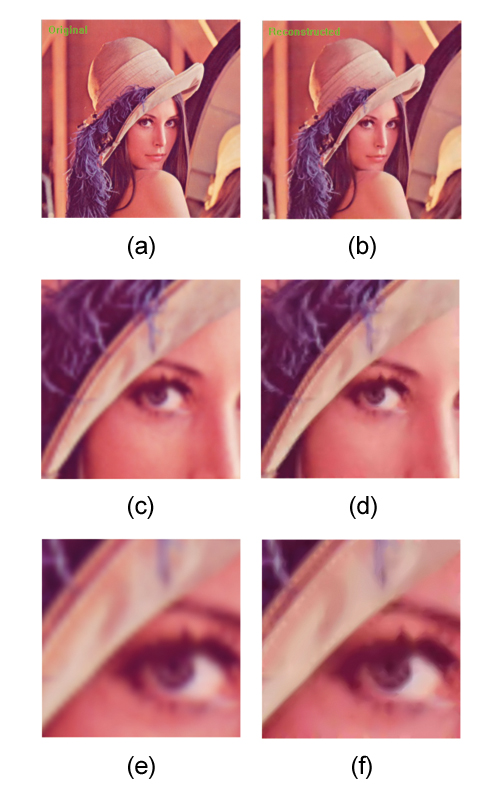
Apart from Figure 1 all the examples showing our interpolation approach are applied to the reconstruction of YUV images with Y at intervals of 10 and UV at intervals of 5. In Figure 9(a) we show an original pixel image (the standard test image 'Lena') and its re-rendered equivalent in Figure 9(b). At intervals of 10 between Y levels the re-render is visually indistinguishable from the original (input spatial resolution 256 x 257). Additionally we have shown in Figure 9(c) and (e) two portions of 'Lena' scaled by 4 and 8 respectively using bilinear interpolation (which is usually preferred in the film industry over higher order methods, because it gives a more 'punchy' image). As one expects the detail becomes more blurred. By comparison we have scaled the control points for the contours in Figure 9(b), again by x 4 and x 8 and rendered these as in Figures 9(d) and(f) where we can see that more detail has been carried into Figure 9(f) than in Figure 9(d).
Figure 9. Rendering 'Lena' image with various techniques (a )Original 'Lena' image , (b) Rendered from contours (x1), (c) Original x4 (bilinear), (d) Contour control points x4, (e) Original x8 (bilinear), (f) Contour control points x8
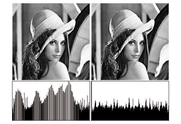
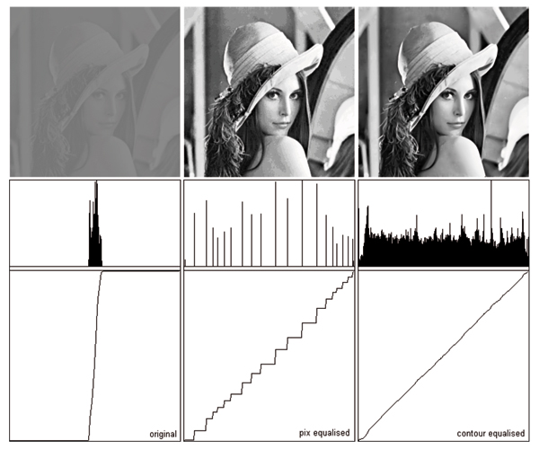
For our second application we chose a different kind of operation, histogram equalisation. The purpose behind histogram equalisation is to adjust pixel values so that each sub-region of the image yields equal energy. Properly histogram-equalised images should show the highest contrast everywhere in the image and this is supported by a rectangular histogram across the range, particularly for the Y component of a YUV image. Unfortunately pixel-based histogram equalisation usually only manages to achieve the sort of result in Figure 10(a). The diffusion interpolating technique however does not require level lines to be associated with integral values although one might start out that way. Instead one could determine what level values would give the nearest to a rectangular histogram. The neatest way of doing this would be to start off with contours of values which vary in powers of 2 around 127, i.e. 127, 63, 191, 31, 47, 159, 223 etc. The 127 contour should partition the image area exactly in half and if not, its value needs to be reassigned to whichever contour comes closest to achieving that partition, if necessary generating contours (levels) to ensure that partitioning proximity.
We re-assign the levels by indexing the inverse function H-1() by the proportion p of pixels actually covered (0 ≤ p ≤ 1). Here H(l) = 2ln(l+1)-8 so H-1(p) = p*28 - 1 (for an 8-bit per primary quantised colour space). Figure 10 shows the results of performing histogram equalisation in this way. Here the first row shows the resultant images and the second row shows the corresponding histograms. It is clear that the right hand image Figure 10(b) has the strongest contrast enhancement of the two images and in particular lacks the artefacts of the left image Figure 10(a) which are in the main caused by the gaps introduced by pixel reassignment in the histogram.
Vector formats for photographic images have been studied for various purposes since the mid 1970s and there are broadly two approaches, the morphological approach which in effect requires every individual quantisation of the colour level to be represented, and the topological approach which attempts to model the isosurface as economically as possible. Level sets, as we have used them here, are a bridge between the two approaches and can benefit from results in either. Many image manipulation operations on this form are both simpler and seem to give better results (as here, warping and histogram equalisation) than their raster equivalents. One kind of transformation is particularly straightforward, that of varying the colour depth resolution in the resulting image. This is because the final samples for the observed image are calculated as a convolution of samples into the continuous field and these need then to be quantised to whatever colour depth is required. Thus the vector form is independent both of spatial and colour depth resolutions in the original input.
However there are residual problems with the vector approach which can be summarised in terms of conversion speed and file size. Conversion times in and out of the vector format are approximately linear with input image size although it is known that images with a lot of high frequency detail take longer to encode and decode than images with a more usual distribution of frequencies. For example the 'mandrill' image (another one of the standard test set) takes twice as long to encode as 'Lena'. On a 500MHz PC 'Lena' at 256 x 257 took 15 seconds to encode and 20 seconds to decode, but this is without any graphics acceleration assist. The codec is (by intention) wellsuited to streaming and parallelisation. Our view is that, given the degree of support available for graphics processes, these times will be significantly improved in practice. On the other hand the fixed contour level setting strategy resulted in file sizes 10x larger than their pixel equivalents which we did not attempt to address in the work being reported here. However, the results of Lindeberg[ Lin98 ] suggest we have been far too conservative in fixing the local resolution of contour segments in smooth areas. If we compute a resolution measure which scales with local smoothness we should be able to significantly reduce the number of segments per contour. We have also (knowingly) been far too conservative in the numbers of contours we find, possibly by as much as a factor of 20, but it will take a (much more complex) adaptive encoder to find the local optima. Compression is an obvious focus for future work.
Figure 12. (top to bottom): (a) Seagull (original image) with neck feather detail from below beak (b) Vectorised image render with same feather region
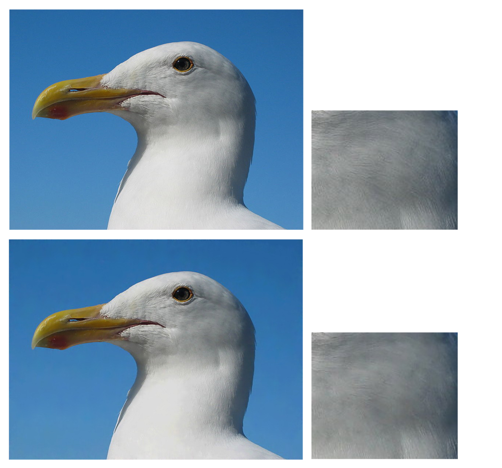
Our original concern was to be able to reproduce photographic images from contour form so that they looked visually indistinguishable from the original. In this we were generally successful. A particularly demanding example is shown in Figure 12 where a photograph of a seagull, Figure 12(a) has been vectorised and decoded again using the exact regime described in this paper. While the results impressed us they nevertheless show that the method of setting fixed contour levels to find is not perfect (the insets of the same regions in Figure 12(b) and 12(d) which are double image size differ visibly).
Reliably better results could be obtained with an adaptive encoder which starts as we have done here by encoding contour 127 then splitting the intervals on either side etc. Such an adaptive encoder (e.g. [ PW06 ]) would maintain a test render and only split an interval further if the pre-render resulted in pixel values falling outside the assumed error bounds around the original pixels. Where this condition happened locally, a local decision to subdivide further could be taken. We estimate that such a codec would take twice as long to encode as our fixed-level encoder. It would take considerably less time to decode, although this time would be more image-dependent than before. File size should be significantly improved also. The gains here also depend on the noise-estimation method used as well as the extent to which the diffusion process mimics the expected variation of pixels values within a contour footprint. Here there are a number of possible improvements to be made.
The main improvement is to use a standard level set
approach [
Set99
] of adding or subtracting (depending on
the sign convention used) the traversal speed of the level
line with a (usually) small amount, calculated as (say) 0.01
x curvature, where curvature is calculated as
 . This
has the effect of smoothing out 'shocks' or discontinuities
in the evolving line, which is a common problem in
interpolating systems [
Ree81
]. (We note also that loops
are another problem with 2D interpolators but the rules for interpreting Level Set solutions explicitly
precludes these under the 'weakest solution' rule;
instead the loop is cut off at a point which often leaves a
visible shock.) Shocks also arise when two advancing
fronts intersect one another, as in Figure 8(e) and (f)
but again the'weakest solution' [
Set99
] applies to
determine a single front. Again the foregoing modification
smoothes away the discontinuities, but the calculated
indices are no longer computed from wholly linear
(Euclidean) distance values. This would only normally be
done away from edges so requires a separate edge
detection process to work properly. It is also possible to
manipulate these indices further so that tangents in the
trajectories of index values are matched across contour
boundaries to achieve G1
continuity (C1
can be achieved
with greater difficulty, typically as a post-process if
needed after establishing G1
). While we would expect
an improvement in image quality (and a matching
improvement in file size) by these measures, such
improvements are usually visually unnoticeable in an
unwarped image.
Our motivation for this work has been based on the intuition that contours will commonly follow the features of objects in the image. We hope in the future to be able to show that 'difficult' operations like matte-pulling and hole-filling will be enhanced by vector formats in addition to the processes whose enhancement we have already demonstrated. Image re-sizing is such an example where the vector format can be exploited to define localised warps aimed at preserving the slope angle at edges. This has the effect of retaining feature sharpness but vector image resizing under various regimes is potentially the subject of an entire paper in itself, so, despite its importance to some industries, this has not been discussed here.
What we have shown already is that there is a viable continuous image format and that it can be used for some conventional operations which are not handled easily in sampled formats. Moreover, while the representation cannot reveal more detail than in the original sampled image, it does offer a robust model of that image, with all the advantages of being able to render it at different qualities for different devices. It thus has the advantages that SVG offers for graphical pictures but with the ability to deliver the full quality of photographically-captured images.
This paper describes a vectorised image codec which finds contours for non-consecutive quantisations and fills them using a simple-seeming diffusion process during rendering. This two-part process turns out to be surprisingly powerful, allowing full control of the continuity of the rendered isosurface, for example not attempting to enforce more than G0 continuity at edges, although we have not demonstrated this in examples here. We are aware that there is considerable scope for improvement of the codec although the results we obtained here demonstrate or the first time near-perfect reproductions of most photographic images from contour maps. Given the multiple potentials of the approach and given the fact that the 'traditional' objections to vector artwork seem to be melting away we argue that this whole approach to image-making, which banish pixels from anything beyond external representations, deserves closer scrutiny and further work.
We acknowledge funding from the Scottish Enterprise Proof-of-Concept Plus programme and wish especially to acknowledge the work of Peter Balch (Analogue Information Systems Ltd) who implemented the code from which the examples to this paper were produced. We thank the referees for their helpful comments. The photograph of the Western Gull (Larus occidentalis), taken by Dschwen, was downloaded from Wikimedia Commons and is used here under the conditions of the Free Software Foundation's GNU Free Documentation License, Version 1.2 and the Creative Commons Attribution ShareAlike 3.0 licence.
In practice most of the following equations break down in the case of extreme conditions on the numbers of infinitesimal points inside a given footprint() so we say that ℵ(footprint(R)) >> 1 everywhere (ℵ stands for ‘cardinality’ or number of members of the set). There is no such restriction on S. We note also that we have slipped from using the terms R, S for borders to the regions enclosed by these borders, and this is distinguished in the following treatment.
We start by defining lines in terms of the adjacency of infinitesimal points, then define special lines, notably geodesics, which gives minimal distances. Finally we derive dist(,) in terms of geodesics in the plane.
So, the adjacency or (directly) reachable relation ↔ between infinitesimal points a and b in (any) Cartesian region R is defined using Euclidean distance

as follows:
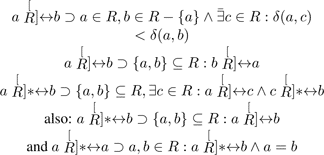
If R is a simply connected region, then

In other words p is reachable from every other member of R, and viceversa. Here the superimposed star symbol denotes Kleene closure.
A continuous line lR is a proper, partially ordered subset of a closed region R defined in terms of the union of a chain of overlapping local regions rR(a) ⊆ lR , so lR ⊂ R and is defined as follows (we drop the appended R when it is unambiguous to do so):


Lines are connected unordered lists of points. A member of the set will have exactly two or three adjacent points. A line may be open or closed, depending on whether it has zero or two end-points in the end-point set Pl for the list lR .

If ℵ(Pl) = 0, line l is closed, otherwise (ℵ(Pl) = 2) line l is open, with two end-points.
A closed line lR partitions a connected region R (here the equivalence class defined by inside(()) into a simple region R'(lR), the border lR ⊃ R, and

The border lR is thus explicitly excluded from being part of the region R as only points unambiguously inside count. Care has to be taken when deciding when the border points are going to be included in a set or partition,or not.
These formulae define the length function ⧼,⧽() along a line in terms of Euclidean distances δ(,) between the smallest line segments. Lengths, here, imply that points are organised as lines (as above).

The function geo(,) defines a geodesic, the shortest distance between two points inside a closed, finite, irregular boundary.

We can now define the (polymorphic) morphological distance function dist(,) between two points a, b:

also between a point a in a closed regionR and a closed region S enclosed by R:

[ASNA87] An Automatic Interpolation Method of Gray-Valued Images Utilising Density Contour Lines, Proc. Eurographics '87, 1987, pp. 405—421, isbn 0-387-90839-0.
[Bli05] What is a pixel?, IEEE CG and A, (2005), no. 5, September/October, 82—87, issn 0272-1716.
[DHH02] SVG: Scalable Vector Graphics Tutorial, WWW2002 Conference, Hawaii, USA, 2002, http://www.w3.org/2002/Talks/www2002-svgtut-ih/ .
[Lin98] Edge Detection and Ridge Detection with Automatic Scale Selection, Int. J. Comp. Vis., (1998), no. 2, 117—154, issn 0920-5691.
[Mat75] Random Sets and Integral Geometry, 1975, Wiley, NY, isbn 0-471-57621-2.
[NAT83] Coding Method of Gray-Valued Image by Density Contour Lines, Tech. Rep. I.E.C.E. Japan IE83-74, 1983, pp. 1—6.
[OBB07] Structure Preserving Manipulation of Photographs, Proc. NPAR 2007, 2007, pp. 103—110, isbn 978-1-59593-624-0.
[OBW08] Diffusion curves: a vector representation for smooth-shaded images, ACM Transactions on Graphics (Proceedings of SIGGRAPH 2008), (2008), no. 3, Article 92, issn 0730-0301.
[PB06] Object-Based Vectorisation for Interactive Image Editing, The Visual Computer, (2006), no. 9-11, 661—670, issn 0178-2789.
[PW06] Method for Image Processing and Vectorisation, UK Patent application, July 2006, GB06131199.9.
[Ree81] In-betweening for Computer Animation Utilising Moving Point Constraints, ACM Computer Graphics (Proc SIGGRAPH 81), (1981), no. 3, 263—269, isbn 0-89791-045-1.
[Sch90] An Algorithm for Automatically Fitting Digitised Curves, Grapics Gems, A. Glassner (Ed.), 1990, Academic Press, isbn 0-12-286165-5.
[Set99] Level Set methods and Fast Marching Methods. Second Edition, Cambridge University Press, Cambridge, UK, 1999, isbn 521645573.
[CRM96] A Simple Edge-Sensitive Image Interpolation Filter, Proc. Int. Conf. Image Processing, 1996, pp. 711—714.
[SLW07] Image Vectorisation using Optimized Gradient Meshes, ACM TOG, (2007), no. 3, 11—17, issn 0730-0301.
[Smi95] A Pixel is Not a Little Square, A Pixel is Not a Little Square, A Pixel is Not a Little Square! (And a Voxel is Not a Little Cube), Technical Memo 6, Microsoft Research, 1995.
[Vin93] Morphological Grayscale Reconstruction in Image Analysis: Applications and Efficient Algorithms, IEEE Trans. Image Processing, (1993), no. 2, 176—201, issn 1057-7149.
[VWV01] Real-Time Modelled Drawing and Manipulation of Stylised Characters in a Cartoon Animation Context, Proc. IASTED International Conference on Computer Graphics and Imaging (CGIM 2001), 2001, pp. 44—49.
[WW67] Concepts and Applications - Spatial order, Harvard papers in Theoretical Geography, (1967), no. 1.
Fulltext 
-
 Volltext als PDF
(
Size
7.2 MB
)
License 
Any party may pass on this Work by electronic means and make it available for download under the terms and conditions of the Digital Peer Publishing License. The text of the license may be accessed and retrieved at http://www.dipp.nrw.de/lizenzen/dppl/dppl/DPPL_v2_en_06-2004.html.
Recommended citation 
James W. Patterson, C. D. Taylor, and P. J. Willis, Constructing And Rendering Vectorised Photographic Images. JVRB - Journal of Virtual Reality and Broadcasting, 9(2012), no. 3. (urn:nbn:de:0009-6-32713)
Please provide the exact URL and date of your last visit when citing this article.
