GI VR/AR 2011
Generating and Rendering Large Scale Tiled Plant Populations
urn:nbn:de:0009-6-36322
Abstract
Generating and visualizing large areas of vegetation that look natural makes terrain surfaces much more realistic. However, this is a challenging field in computer graphics, because ecological systems are complex and visually appealing plant models are geometrically detailed. This work presents Silva (System for the Instantiation of Large Vegetated Areas), a system to generate and visualize large vegetated areas based on the ecological surrounding. Silva generates vegetation on Wang-tiles with associated reusable distributions enabling multi-level instantiation. This paper presents a method to generate Poisson Disc Distributions (PDDs) with variable radii on Wang-tile sets (without a global optimization) that is able to generate seamless tilings. Because Silva has a freely configurable generation pipeline and can consider plant neighborhoods it is able to incorporate arbitrary abiotic and biotic components during generation. Based on multi-level instancing and nested kd-trees, the distributions on the Wang-tiles allow their acceleration structures to be reused during visualization. This enables Silva to visualize large vegetated areas of several hundred square kilometers with low render times and a small memory footprint.
Keywords: Ecosystem simulation, Wang-tiles, Instantiation, Poisson Disc Distribution, Terrain rendering, Ray Tracing
Keywords: Ecosystem simulation, Wang-tiles, Instantiation, Poisson Disc Distribution, Terrain rendering, Ray Tracing
SWD: Simulation, Ray tracing, Rendering
Modern geographic information systems are able to cope with extremely large highly detailed data sets in real time that are available for almost all areas of the world. For planning and simulation three-dimensional visualization of these data sets is gaining more and more importance. Since plants are a crucial component of almost all small scale landscapes the realism of these visualizations can be highly increased by visualizing the predominant vegetation.
However, plants are complex structures with complex ramifications including bark and detailed foliage. Therefore, 3D plant models often consist of thousands of triangles. In order to reduce the data's complexity during the visualization different data can be reused using instantiation. Instantiation can be used on different levels, from single leaves up to whole reusable populations, i.e. it can be applied hierarchically on multiple levels (multi-level instancing). Based on the work by Dietrich et al. [ DMS06 ] for the visualization of vegetation we propose a method for the automatic generation of vegetation with regard to the instantiation schemes used during visualization.
Due to their rectangular shape Wang-tiles have proven to be well suited to easily generate reusable patterns for texture synthesis and object distributions [ CSHD03 ]. In [ DMS06 ] plant distributions on Wang-tiles are reused throughout the scene. This makes it possible to reuse the accelerating data structures needed for rendering.
However, instantiating is not only used for parts of the population but also for the plant models themselves. Silva allows for the generation of reusable plant populations on such instantiable Wang-tile sets to provide vegetation that can be instantiated on multiple levels.
The goal of an ecosystem simulation is to find a production algorithm that allows generating a plausible plant population under consideration of the ecological surrounding. In general, a first naive approach is to distribute plants randomly using PDDs. Recent publications to generate PDDs, like [ DH06 ] or [ Jon06 ], generate distributions where the distance between the sites is fixed. These distributions are well suited for sampling but are not suited for the generation of plant populations since the maximum radius of the plants foliage or comose radii are highly varying in nature. A good overview of other methods to generate PDDs is [ LD08 ].
Entirely random distributions of plants are usually considered implausible for large areas as they do not consider ecological components and plant neighborhoods. Commercial products like Vue [ E-o10 ], Worldbuilder [ DE10 ], SpeedTree [ IDV11 ] or the vegetation tool of the CryENGINE 3 [ Cry12 ] offer different methods to "design" vegetation. There, plants are placed by painting or specifying regions where single or small sets of plants are placed randomly. Usually these regions are specified by 2D density maps. However, these tools do not allow to automatically generate the vegetation based on predominant ecological components. These systems provide no interface to be coupled to real world data. In addition, the size of the landscapes is limited because they do not support to reuse large-scale distributions. In order to visualize dense vegetation on areas of a couple of thousand square kilometers, instantiation schemes for plant models and distributions must be applied.
One simulation approach that incorporates the ecological surrounding is [ DHL98 ]. Starting from an initial distribution, plants grow and compete with each other. For each plant one value is computed describing its ecological vigor in relation to the predominant ecological components. If two plants demand the same resources due to their growth, i.e. when their sites representing their region of influence intersect, the weaker one dies. In addition to this thinning, new plants are added over time or die because of their age. However, this model does not consider the plants' distances to one another.
Neighboring plants may have a greater influence on each other than on the ones farther away but are not necessarily lethal for one or the other. Thus, the influence of neighboring plants must be distributed distance weighted. This is considered in the FON (Field of Neighborhoods) model [ BH00 ], first introduced for mangrove forests.
An even more elaborate system using a FON simulation is [ AD05 ]. In this system neighborhoods of different sized species are examined. This system proposes a fixed function pipeline for the simulation. The ideas of [ AD05 ] are extended in [ BAMJ11 ] for urban areas, where the simulation methods are altered to support more controlled areas within an urban environment. Some of these methods can be modeled with Silva as well. However, all these approaches are simulations over time allowing plants to grow and have varying positions during the simulation. There is no way to map the simulation results onto a smaller set of Wang-tiles that is able to regenerate the simulation results by creating an aperiodic tiling.
A more generic approach to describe growth and simulations for ecosystem is realized in OpenAlea [ Ope10 ]. In [ Ope10 ] arbitrary models can be described via connectable simulation modules using a graphical interface. OpenAlea uses Lindenmayer-Systems (L-Systems) [ PL90, Chap.1], which are a common tool to describe growth of single plants to whole populations [ DL05, p. 65]. In another system GroIMP [ Fac10 ] rule-based modeling using a relational growth grammar (RGG) expressed through a Java based domain specific language called XL is used. Both systems allow for simulations on very small areas and do not support the generation of reusable population components.
In order to visualize 3D plant populations ray tracing of such natural scenes has been an active research topic since more than twenty years. One major problem is the vast amount of geometric data that needs to be processed while displaying large plant population, e.g. forests. Early systems like [ PKGH97 ] that could visualize large amounts of data exceeding main memory always used caching and paging methods. However, these systems are not suited for an interactive visualization of a large number of plant models, do not reuse data during visualization and suffer from the bandwidth limitations of the memory hierarchy.
Another way to display large plant populations is to change their representation by using simpler primitives. One framework that is based on OpenRT [ Ope07 ] was introduced in 2005 by Dietrich et al. [ DCDS05 ]. There the complex polygonal plant models are represented by simple point and line primitives. The largest population displayed by the system was on an area of 300 m x 300 m (see [ DMS06 ]).
The idea of the method used by Silva is reusing positions of sub-populations and their accelerating data structures by using multi-level instancing and Wang-tiles. This is based on the method proposed by Dietrich et al. [ DMS06 ]. In [ DMS06 ] a tiling of the scene using Wang-tiles with PDDs is used to construct a set of nested acceleration structures. This allows to reuse the distribution of the plants represented by the PDDs on the tiles and the acceleration structures constructed for them, throughout the scene. In [ DMS06 ] the plants that are visualized on each Wang-tile are determined at the visualization's run-time. This only allows thinning out thepopulation based on the terrains height. In addition [ DMS06 ] uses a pregenerated fix tile set with fixed radii for each site of the PDD. This usually does not lead to realistic results because the plants seem to be too even in size and too evenly spaced. Therefore, more elaborate simulation methods for the tiles and an automatic generation of PDDs on Wang-tiles with varying radii are necessary. However, combining multi-level instancing with global simulation methods in a way that the simulation yields reusable distributions is challenging. Starting from a global simulation of the whole population one has to map the results to a smaller set of Wang-tiles, that is able to regenerate the initial results as accuratly as possible.
In [ AD06 ] a method is introduced that works with sets of Wang-tile sets containing distributions with varying density. These sets of sets can then be used to generate consistent tilings. However, for large areas one needs many of such small tiles. In addition, by considering sets of Wang-tile sets the number of tiles largely increases. The overhead of the system for the construction of acceleration structures for rendering in advance for all tiles is too large.
Therefore, there is a need to develop methods that combine instancing techniques using small Wang-tile set with an elaborate ecosystem simulation. One method is introduced by Silva.
The main idea of Silva is using hierarchical multi-level instancing as proposed by [ DMS06 ]. A small set of Wang-tiles is used to aperiodically tile a larger polygonal terrain model. Each of the Wang-tiles contains a pregenerated PDD where each site of the PDD corresponds to one plant. This allows to build and reuse nested spatial indexing structures (here kd-trees) to accelerate rendering. On the highest level a kd-tree is constructed over all Wang-tiles of the aperiodically tiled terrain. Each of its leafs holds an index to the smaller set of Wang-tiles. For each of the Wang-tiles a kd-tree can be built over all sites on that tile. With the overall position in the tiling and the site's id on the individual tile the simulation results can be queried to determine the plant's acceleration structure for that plant which will most likely grow on that specify position (multi-level instancing).
Our contributions is a method to create Wang-tiles with PDDs of varying radius for vegetation generation such that it enables the generation of seamless tilings without global optimization. Wang-tiles with PDDs of varying radius create much more realistic looking plant distributions since plants in nature are different sized as well. In addition we introduce a simple graph-based view on the PDDs corner problem and a way to determine plants in a tile's corner that can be discarded during the visualization. Besides the PDD generation we propose a new highly configurable plant generation system which allows for describing local influences taking the site related abiotic and neighborhood relations into account. Fig. 1 gives an overview of the overall system.
Figure 1. Overview of Silva showing the two main modules SilvaSim and SilvaVis, as well as their inputs and outputs.
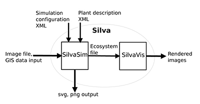
Silva is split into two modules SilvaSim and SilvaVis: SilvaSim can be used to generate naturally looking plant distributions based on arbitrary ecological components out of an a-priori distribution on Wang-tiles. To do so, Wang-tile sets with Poisson Disc Distributions (PDDs) are generated with varying radii. Afterwards, a detailed vegetation generation is performed using a highly configurable generation pipeline as preprocessing. To specify parameters for the simulation SilvaSim uses XML configuration files. In addition the ecosystem can be described using rasterized image or vector graphics file formats. SilvaSim outputs an ecosystem file containing the Wang-tiles, the tiling itself, and the individual instances of the plants to be used. These files can be rendered with SilvaVis using a nested kd-tree hierarchy as in [ DMS06 ]. We render the scene with ray tracing using RTfact [ SG08 ], the ray tracing framework developed at Saarland University. In the next Section 4 we take a closer look at SilvaSim. Sec. 5 deals with the visualization of the simulation's results using SilvaVis.
SilvaSim creates tiles with PDDs, tiles the whole terrain and determines for each individual site on each tile of the tiling which plant is most likely to grow on that position. Using tilings with PDDs has some disadvantages:
-
Plant positions cannot be individually generated and placed on the whole area but are dependent on the position on the corresponding tiles. The positions and the radii of the sites on the tiles are fixed.
-
Plant species are dependent on the radii of the sites that are generated on the tile. On one hand smaller plants can be placed in large sites, either by choosing generally small plant species for a specific site or by scaling plants below this sites radius. However, this yields a smaller density of the overall vegetation, because then there is more space between neighboring sites. On the other hand it is not possible to place larger scaled plant models in smaller sites without an intersection of neighboring plants.
In contrast to [ DMS06 ], where the specific plants are determined during the visualization's runtime, SilvaSim uses an elaborate preprocessing in order to generate more natural looking distributions based on the ecological surrounding. A generation of instantiatable vegetation using Wang-tiles can in principle be performed bottom-up or top-down.
-
Bottom-up: Starting from a simulation of the whole area to be covered, the results need to be broken down to a smaller set of Wang-tiles that is able to regenerate the simulation results.
-
Top-down: Starting from the tiles with pregenerated PDDs the whole area is tiled. Afterwards, the plants need to be selected according to the fix sites' radii and positions given by the tiling.
The problem of the bottom-up approach is finding the smaller tile set that is able to regenerate the simulated plant population. This can be seen as a compression of an input signal, i.e. the simulation results, where a smaller set of base function, the Wang-tiles, need to be found that are able to reconstruct the input signal. However, such compression is a computationally demanding task since all possible PDDs and tile sets need to be examined to determine how good they regenerate the simulation results. In addition this prevents the on-demand generation of the vegetation. In principle, the selection process of the top-down approach can be performed at run time. SilvaSim uses a top-down approach. Starting from a tiling of the whole scene, plants for each individual fix site on each tile are determined.
The module SilvaSim consists of different components. The core of the system is a highly configurable pipeline where the user can specify how different plants interact with their environment and influence neighboring ones. A rough sketch of the pipeline is as follows:
Since the generation of aperiodic tilings is well known and suitable Wang-tile sets are given (Silva uses a 18 tile Wang-set with six colors) we only give some more detailed insights into the steps 1, 3, 4 and 5 of the generation.
As first step in the simulation the Wang-tile sets need to be filled with PDDs. It is important to ensure that the Wang-tiles are able to build up seamless tilings, with PDDs that keep their density along the seams. Since we do not consider PDDs with a fix radius but varying radii for the sites, a relaxation of the PDDs of Wang-tiles using Lloyd's method [ MF92 ] with Voronoi-diagrams is not possible. Using Apollonius-graphs, i.e. weighted Voronoi regions, is computationally expensive. However, the method proposed here enables to generate suitable tile sets with PDDs that allow seamless tilings without a global optimization. The main idea is filling the tiles with respect to the others in the set. Starting with a PDD on one tile the sites in the edge regions are copied to the tiles that have the same edge color for that region in the same direction and next to the tiles edge regions that have matching opposing edges. This process is shown in Fig. 2. Algorithm 1 gives an overview of the generation of the initial PDDs.
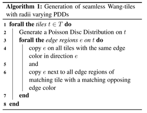
Figure 2. One step of Alg. 1 to generate Wang-tile sets that allow to generate seamless tilings with radii varying PDDs. The edge region of the first tile in one direction is copied to all other tiles (only three shown) in the set.

An edge region contains all sites that are at most two times the maximal radii away from the edge. It is important to start with tiles that have different colors on all edges. Otherwise a position that is close to e.g. the north edge would influence the south edge of the same tile. Similar problems occur with small tile sets with only a couple of colors. However, the method works well with an 18-tile set with six colors. This set is sufficient for finding a traversal order so that we can start with tiles that have different colors on all edges and process the ones that have the same edge colors later on, when their edge regions were already filled by processing the previous ones. Even though we copy edge regions to tiles with the same edge color in the same direction and thus create a small part that could potentially be repetitive along the tile seams in a tiling, these parts are not visible in practice since the edge regions are extremely small. In addition copied tile seams and edge regions simply vanish in the nature of the aperiodicity of the tiling. Also note that we do not copy actual geometry of a plant but only positions where plants potentially grow. The simulation later on decides which plant grows on which site on which tile within the scene's tiling.
The corners need a special treatment since we copy overlapping edge regions and due to the corner problem of Wang-tiles in general. One approach to solve intersections within the corner regions is proposed in Sec. 4.4.
The generation in SilvaSim starts by performing a local soil evaluation. The goal of the simulation is to determine the plant candidates for each site that are mostlikely to grow on their respective location on a certain tile on a certain tile position within the tiling. Here we work on a global scale considering each site in a tiling of the whole scene. In the local soil evaluation only the abiotic surrounding by altering individual growth probabilities is considered. Therefore, SilvaSim computes a scalar growth probability for each site for all plants. Each plant used in the scene is specified by a set of Properties which describe how plants respond to certain ecological components. Each Property yields a scalar floating point number between 0 and 1. Evaluators link these Properties to data fields describing the ecosystem. These Evaluators are then processed in a pipeline yielding scalar growth probability for each site for all plants. To start the simulation we need to specify the ecosystem. Sec. 4.2.1 shows how plant species for the individual scene can be specified using Properties. In Sec. 4.2.2 we show how the ecosystem can be modeled, whereas finally Sec. 4.2.3 shows how the simulation is performed using the Evaluator-Network.
Each plant species can be specified using Properties that describe how a plant species reacts to specific ecological components (e.g. height, soil moisture, nitrogen values, etc.). A response behavior is described by a floating point number ranging from 0 to1. This could either be a constant specified by a Constant-Property for the plant or it could be the result of a complex function e.g. Gauss- or Bézier-Property. One main goal in the development of SilvaSim was to make it highly configurable. SilvaSim supports a variety of Properties and ways to describe them. A simulation can be specified using XML. The following XML fragment shows the assignment of a MinMax property to one plant specifying a range of moisture levels where a plant is likely to grow.

Silva offers different Properties that can be used to specify plant models ranging from simple constants or value ranges to complex response functions.
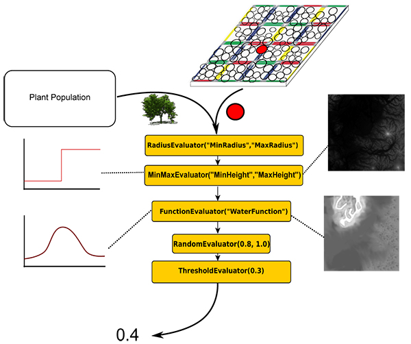
The ecosystem itself consists of an arbitrary set of data fields, which describe the distribution of the ecological parameters. These data fields usually are rasterized greyscale images or are coming from vector file formats. By specifying Evaluators these data fields can be linked to the Properties giving a description how the data fields are evaluated against the properties. Silva offers many different Evaluators. The RadiusEvaluator determines if a geometrical plant model can be scaled to the given sites' size on a specific location. The MinMaxEvaluator allows the specification of value ranges to specify if plants are viable in a certain parameter range, e.g. the height or moisture level. The FunctionEvaluator can be used to evaluate response Function-Properties based on the prevailing ecological parameters. This way e.g. a thinning of the populations density can be described based on height, nutrition levels or soil moisture. Similar the GradientEvaluator allows for describing thinning out of certain plants by specifying a linear gradient that reduces a plant's viability in a certain region.
The Properties to be accessed during the simulation are linked to a data field using the properties name within the Evaluators. The following XML fragment shows the specification of a data field and a simple evaluator which links the data field to the plant's Property named MinMaxWater

This MinMaxEvaluator links the Property MinMaxWater to the data field Waterfield given by a png file. The Property MinMaxWater describes a range of moisture levels individually for each plant. In the process of the evaluation of the MinMaxEvaluator the system looks up the interpolated moisture level given by our data field for the current site's position and checks for each plant if it is within the range of the Property given by MinMaxWater. Since the attribute optimum is set to false, we do not compute the distance to the theoretical optimum given by the average min/max value of the Property but simply yield a probability of either 0 or 1. Since the attribute lethal is set to true, we allow for a probability of 0 to become effective and remove all plants not in range from the set of possible candidates.
After we have specified the ecosystem by providing two XML files we can begin with the simulation. Starting from a global tiling of the scene, SilvaSim processes each individual site of the PDD on each tile of the tiling. For each site SilvaSim alters the scalar growth probabilities by evaluating the evaluator pipeline for all individual species in parallel. In order to compute a new growth probability, consecutive nodes within the evaluator pipeline have access to the results of all predecessors and can interpret these growth probabilities as a series of multiplications. However, simply multiplying consecutive probabilities might lead to a system that is too erosive, meaning that too many plants are discarded. In addition, this makes it hard for the user to predict how the system reacts to slight changes of the data fields. Additionally, the range of the growth probabilities might be highly varying. Therefore, SilvaSim offers a NormalizeEvaluator, which normalizes the scalar growth probabilities to a range between [0,1]. Since we have to normalize using the probabilities of all species and all sites and since we do process in parallel we have to use a barrier in the NormalizeEvaluator to ensure, that all pipelines for all sites have been evaluated up to that evaluator. We now normalize the growth probability used in all consecutive Evaluators by using the maximal overall growth probability computed up to that point.
A single Evaluator that evaluates to zero leads to a growth probability of zero for the whole pipeline. One alternative to the simple multiplication approach is the representation of the growth probabilities of consecutive evaluators as the length of a multidimensional vector. Each component of the vector is the outcome of one individual evaluator in the pipeline. This way the system is less erosive since a zero within the vector does not lead to a length of zero for the whole vector. However, some parameters of the ecosystem are lethal no matter what. The user can decide if the results of consecutive nodes are evaluated by means of multiplication or as vector length and if single parameters are lethal or not. Fig. 3 shows an exemplary pipeline.
After the evaluation of the local soil factor each site has a list of potential plants to be chosen and their growth probabilities respectively.
Figure 3. Exemplary pipeline to determine plants growth probabilities for each site on each tile of the tiling based solely on the abiotic surrounding
Right now the list of potential plants for each site and their growth probabilities are solely based on the local abiotic components but not on the plant's neighborhood. SilvaSim offers a method to take the influences of the neighborhoods, i.e. the biotic components, into account. As in FON-Models this is done using a distance weighted approach.
The aim is to select the plant candidates that are likely to grow in the surrounding of the neighboring ones. Let's assume each plant can have a positive or negative influence on each other plant by distributing distance weighted probabilities to its neighborhood.
Note, that it is important where and with which plant from the list to start. A solution to this problem would have to take a look on all possible combinations of sites and list candidates coming from the local simulation. Checking all possible solutions is too computationally intensive. Therefore, SilvaSim offers an approximation approach. The idea is to sample the set to determine those plants which are most of all determined by the results of the local soil evaluation and use these plants as starting points to distribute distance weighted probabilities. Algorithm 2 shows the core of the method.
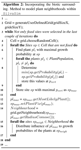
We reduce the problem to smaller grid cells since processing the whole population is computationally demanding for very large scenes. In the first step an uniform, user-defined grid for the whole tiling is created. Afterwards one of the grid cells is chosen randomly. All plant positions that lie within the cell are examined by determining how uniquely they were defined by the local soil evaluation. This is our starting site to distribute distance weighted probabilities. To do so we look at all sites sp in the cell that have not already been processed, i.e. that are not fixed (see Alg. 2, lines 5-8). For each sp we determine the plant candidate pli which has the maximal growth probability based on the results of the local evaluation. With this maximal growth probability we determine the minimal difference between all other growth probabilities of all other plant candidates plj for that site. We compute this value for all sites. The site with the maximal minimal difference value within the cell will be set fixed to the plant that is most likely to grow there. It is most uniquely defined by the local soil evaluation. Because we have set it fixed it can no longer be altered by any further neighborhood operations.
Since the plant species for that site is now known and fix, the plant's region of influence can be computed. The plant's FON-radius is described in the XML file and is now weighted by the scale factor of the current site. This radius can be used to determine the neighboring positions. To find the neighboring sites we utilize the already created grid structure. Within this neighborhood the influence of the fixed plants can be distributed to the plant species not fixed yet. (See Alg. 2, line 14ff)
This method can be applied until the distribution stabilizes, i.e. when more or less all sites are set fixed. Since we start by randomly choosing a grid cell we have to stop when we have only selected fixed sites in the last couple of iterations. This termination criterion, i.e. the number of iterations where only fixed sites were selected, is user-defined. In addition, since we only approximate thecorrect results we can use this approach for several passes to come closer to the overall correct result. In each new pass all plants even the ones that were set fixed in the last pass can be altered. We can terminate when the distribution more or less stabilizes that means the plant candidates with the maximal growth probabilities for each site did not change in the current pass or use a user defined upper bound. In practice specifying a small upper bound usually is sufficient since nature is highly varying anyways and the benefit from having it run more passed is not noticeable in the rendered image.
The algorithm to fill the tiles with PDDs yields tiles that have no intersecting sites along the tiles edges when used in the creation of an aperiodic tiling. However, due to the copy operations of the tile edges and the corner problem of the PDDs on Wang-tiles in general, intersections in the corner regions can occur (see Sec. 4.1). Fig. 4(a) shows four tiles and the intersections (for the corner problem). Some intersecting sites already have been eliminated, i.e. they have no plant model attached, by the simulation and hence are not displayed. However, it might be the case that some intersecting sites remain.
Figure 4. Graph-based visualization of the intersections across tiles (corner problem): (a) The corner problem of Wang-tilings; (b) intersecting sites across tiles and (c) mapping to a graph.
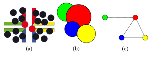
Intersecting sites (see Fig. 4(b)) can be described as a graph G = (V,E) with an edge between each intersecting ones (see Fig. 4(c)). We start by creating such a graph for all intersecting sites within each corner region of the tiling. The goal is to delete nodes from the graph until all remaining nodes have a degree of zero. Right now each site has no or a single plant model attached that is most likely to grow there. To remove intersections we want to keep the nodes, which represent sites that have plants attached that are most likely to grow and cover a large area.
During visualization the deleted nodes from the graph will get no plant model attached and thus will not be visualized. We take care of intersections by not deleting them from the tile in terms of trying to find a globally optimal tile set but by not displaying them at run-time. To map this problem to our graph each node gets a weight w(a) based on the following function:

Where p(a) is the growth probability of the plant assigned to the site a. This probability is scaled by the radius of the site to preserve a dense coverage of the vegetation. A correct solution to the problem would be a new graph G', with:

In the graph, each node in V' ⊂ V has a degree of zero and thus has no intersection with any other node. A solution is considered optimal if there exists no other graph G'' = (V'', ∅) where the sum of all the weights w(a) is larger than the sum of weights in G' = (V', ∅).

Hence, we are looking for a configuration of non-intersecting nodes where the covered area and the growth probabilities are maximal. In order to maximize this value without testing all possible solutions of active and inactive sites SilvaSim uses a probabilistic approach. Therefore, an extended node weightwext is computed.
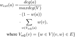
The first part
 considers the number of
intersections within the direct neighborhood. The larger
the degree of the node the more sites it intersects. Hence,
we want to remove nodes first that potentially intersect a
lot of other nodes because it is more likely that the
remaining nodes are then not intersecting. The second part
of the weighting function (1-(w(a))) takes the current
growth probability of this node into account. We want to
remove the nodes that are not very likely to grow at this
position and do eventually cover only a small area. The
following sum over the weight of the direct neighborhood,
i.e. the adjacent nodes, takes the growth probability andthe coverage of the neighboring plants into account. We
want to remove those nodes that intersect with sites
which are very likely to grow and provide a good
coverage.
The algorithm starts by deleting the node where this weight is maximal. After the deletion, all other nodes now having a degree of zero are deleted from the graph. These nodes and thus their respective sites in the PDD no longer intersect any other node and this site and can be rendered. The algorithm continues until all nodes have a degree of zero and accordingly no node is left for each graph.
The results of the simulation with SilvaSim can now be written to a file. This file contains the tile set with the PDDs on it. To allow referencing these sites later on, each site of each PDD on each tile gets assigned a site's ID. Next this file stores the overall tiling of the scene and an array containing the plants as ID most likely to grow according to the generation results for each site ID for each tile of the tiling. These files can then be visualized using the component SilvaVis.
In addition, to allow for a more user-friendly quicker feedback from the simulation the results are output to a svg or png file. This later on enables the designer of the ecosystem to show the results in other modeling tools as a texture on top of the terrain. This way he is able to get a first impression on the overall appearance and the effects of certain parameters of the simulation pipeline on the vegetation more directly.
In this section a method to visualize the ecosystems that were generated by SilvaSim is introduced. The output of SilvaSim is a file that contains a Wang-tile set with PDDs on each tile, a tiling of the whole area and a mapping of tile positions in the tiling and their individual site IDs to plant models. Since the vegetation is given on Wang-tile sets complete distributions can be reused and their according acceleration structures only need to be constructed once. SilvaVis visualizes these files using ray tracing. To do so we follow the approach proposed by Dietrich et al. [ DMS06 ]. We do not apply any geometrical simplification to our tree models but use raw triangle data. The foliage in the tree are quads with alpha mapped leaf textures. An average tree consist of 200k triangles. The implementation is based on RTfact [ SG08 ], the ray tracing framework by Saarland University. For the visualization RTfact was extended with all necessary spatial acceleration structures as well as methods for their construction and intersection. This results in a couple of nested kd-trees, which were implemented using RTfact's unique template architecture.
SilvaVis constructs a hierarchy of kd-trees. On the highest level a 2D kd-tree is built over all tiles of the tiling and the terrain. Therefore, the terrain is tiled with the Wang-tiles based on the tiling coming from SilvaSim. With this tiling the ground primitives of the terrain are subdivided in patches of the same size as the Wang-tiles (see Fig. 5). For the ground primitives of the terrain a regular kd-tree is constructed. This leads to leaf primitives that hold a reference to the kd-tree of the ground primitives and a pointer to one Wang-tile of our set. During the construction of this acceleration structure the subdivision of the leaf primitives, that are the tiles and the terrain primitives, is only performed along the x- and y-axis. The inner nodes store the minimal and maximal heights of the children. The height of a leaf node is computed by the height of the terrain plus the height of the largest tree in the overall population. This information is used during the traversal to hierarchically skip larger parts of the terrain (see [ DMS06 ]).
Figure 5. TerrainTile Kd-tree with a 2x2-tiling. Leaf nodes store a reference to a Wang-tile (W) of the tile set and a kd-tree for the terrain ground primitives (T) of the area covered by the tile
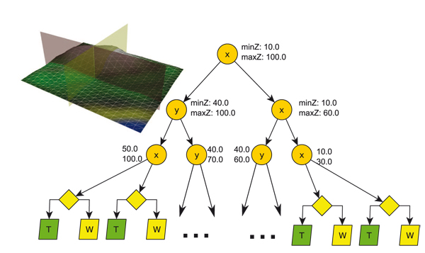
The leaves of this acceleration structure contain nodes that store a pointer to the respective Wang-tile and an acceleration structure for the ground primitives, here a kd-tree. (see Fig. 6).
Each Wang-tile contains a PDD, which represent the plant distribution. Since each of the plant positions on the tiles is fixed, acceleration structures, i.e. kd-trees, for the sites can be constructed (see Fig. 6). The subdivision in the kd-tree construction for the PDDs on the tiles only takes place along the x- and y-axis as well. Because we only subdivided along the x- and y-axis the tree positions can be shifted in the z-direction according to the terrain they are mapped to. To decide which plant model to visualize on a tile at a specific location we can use the ID of the intersected site and the relative position of the intersected tile in the tiling both determined by traversing the upper two of the nested acceleration structures.
Figure 6. Lazy 2D kd-tree of a Wang-tile built over the varying radii PDD. The sites of the PDD can be mapped to arbitrary shaped terrain.
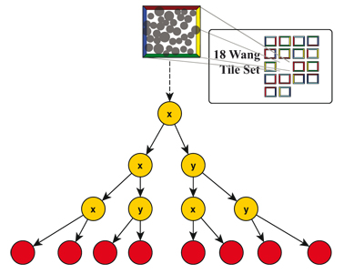
Figure 7. A way to determine the explicit plant instances used for a Wang-tile in the tiling. Based on the TilePosUV and the SiteID the concrete PlantID used at this position can be requested from the simulation results. This PlantID can be used the request the plant model's acceleration structure.
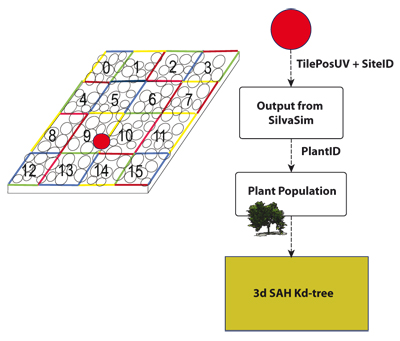
We start the intersection test for a ray by traversing the kd-tree on the highest level. We can skip those parts of the terrain that are not within the view frustum or where the ray is completely above or below the cell's extent in z-direction. When we arrive at a leaf primitive, the deeper structures need to be traversed. The leaf primitives contain a reference to the kd-tree of the Wang-tile from our set and a kd-tree for the ground primitives. Additionally by hitting a leaf we know what tile we have hit in the tiling (TilePosUV). From there we traverse both acceleration structures independently and combine the results.
We load the respective kd-tree according to the referenced Wang-tile. This is the kd-tree that is built over all sites of the PDD. Therefore, we transform the ray from the global space to the local space of the Wang-tile and start traversing. Keep in mind that this tree is only a 2D-tree, meaning that it was subdivided only along the x- and the y-axis because the individual sites can be mapped to arbitrarily shaped terrain. The sites on the Wang-tiles are only placeholders for the plant models. We possibly arrive at a leaf primitive of this inner kd-tree which is a site storing a SiteID. With this SiteID the kd-tree of the plant model that is used at this individual location needs to be loaded. The process to determine the concrete species for the site is shown in Fig. 7. Using the position of the tile (TilePosUV) in the tiling and the ID of the site (SiteID) the concrete ID of the plant species can be requested from the simulation results of SilvaSim. This results in a PlantID that can be used to request the instance of the acceleration structure of the tree model. As in [ DMS06 ] we use a regular kd-tree for the tree models. To traverse this kd-tree we transform the ray from the Wang-tile space to the object space of the tree model. Therefore, we shift the ray according to the z-displacement of the tree based on the position on the terrain (see [ DMS06 ]). Additionally, we slightly rotate the ray (and thus the plant model) based on pseudo-random rotation value computed from the SiteID and the TilePosUV. The intersection result of the ground primitives and the results of the intersection tests from the Wang-tile now can be combined to determine the closest hit point.
Figure 8. Simulation results of the scene UniSB (5km x 5km with a 10 x 10 tiling). Different colors represent different species.
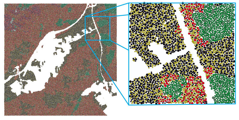
Table 1. Benchmarks of SilvaSim with four test scenes (single threaded).
|
Scene |
Size |
#Tiles |
#Evaluators |
#Active plants |
Time |
|
UniSB |
3km x 3km |
10 x 10 |
7 |
29003 |
16 sec. |
|
UniSB |
6km x 6km |
10 x 10 |
7 |
113481 |
42 sec. |
|
UniSB |
9km x 9km |
10 x 10 |
7 |
252299 |
89 sec. |
|
PugetSound |
10km x 10km |
80 x 80 |
8 |
323565 |
16 sec. |
|
PugetSound |
20km x 20km |
100 x 100 |
8 |
1262512 |
60 sec. |
|
PugetSound |
40km x 40km |
200 x 200 |
8 |
4994147 |
228 sec. |
Table 2. Benchmarks of SilvaVis averaged from 300 frames (without shadows).
|
Scene |
Size |
Tiles |
#Plants |
Tris total |
Time per Frame |
|
UniSB |
3km x 3km |
5 x5 |
35768 |
5.77 ∙ 109 |
3.14 sec. |
|
UniSB |
3km x 3km |
10 x 10 |
36944 |
5.96 ∙ 109 |
3.08 sec. |
|
Puget Sound |
20km x 20km |
100 x 100 |
1262512 |
2.04 ∙ 1011 |
33.7 sec. |
|
Puget Sound |
40km x 40km |
200 x 200 |
4994147 |
8.06 ∙ 1011 |
53.91 sec. |
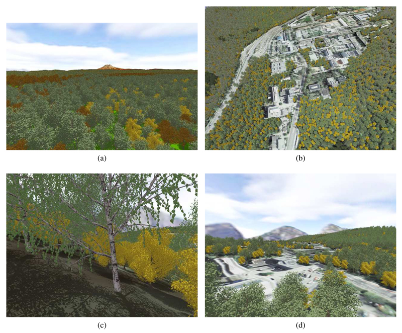
Since the plausibility of a natural distribution cannot be determined without considering real datasets, which were not available, Fig. 8 shows only the result of the simulation. Different colors represent different species. The ones with different shades of green are conifers. The rest are different broadleaf species. Note, that no repeating patterns are visible. Fig. 9 shows some images that where rendered using SilvaVis. The figures show two different test scenes. One is a model of the campus at Saarland University (UniSB) and the other one is a DEM of the Puget Sound data set [ USG10 ] (PugetSound). Fig. 9(b) shows the sample scene UniSB with a 10 x 10 tiling. Fig. 9(c) shows the complexity of the plant models (about 160k triangles per tree).
Figure 9. Figure 9: Renderings from the test scenes PugetSound and UniSB: (a) PugetSound 40km x 40km (flight) ; (b) UniSB 3km x 3km (birds eye view); (c) Puget Sound (close up) and (d) UniSB (flight).
As hardware platform for the benchmarks a shared memory system with two Intel Xeon E5520 CPUs with 24GB RAM running Windows7 was used. Table 1 shows the run times for the generation of the two test scenes with SilvaSim. Since these times are not entirely dependent on the scene′s size but on many factors like, e.g. the depth of the evaluator pipeline, the benchmarks shown only give an idea of the magnitude of typical run times. Please also note, that SilvaSim was not especially optimized or parallelized since the focus on the simulation was more on its configurability.
Table 2 shows the run times of the visualization with SilvaVis. Smaller tiles usually lead to better render times for most viewing angles. This way the traversal can be stopped in higher levels within the nested acceleration structure. This allows for faster render times even for very large scenes. In contrast to [ DMS06 ] where an almost constant run time for larger scenes was achieved once the systems was saturated by a certain scene complexity this is not true for Silva. Once the scene size is large enough the system is able to skip larger parts of the scene by simply traversing the first acceleration structure over the tiles. As in [ DMS06 ] the run time does not increase linearly with the scene′s size within Silva. Even though RTfact generally performs better than the Ray Tracing System OpenRT, which was used for [ DMS06 ] we could not achieve the same render times. The reason for the overall difference compared to [ DMS06 ] is that RTfact has a problem with the evaluation of the alpha mapped leaf textures of the plant models. In case a ray hits such a leaf, RTfact needs to stop traversing, switch over to the shader code and start generating entirely new rays in case of transparency. This is a design decision within a ray tracer whether it does perform some shading, i.e. the lookup of the alpha values within the traversal, or not. In the upcoming releases of RTfact a tighter coupling between shading and traversing was planned. Due to the framework character and the generic programming paradigms used by RTfact in the current version this could not be realized transparently inside an intersector without losing some of its framework character which enables simple exchange of parts of the underlying acceleration structure. However, in contrast to [ DMS06 ] which uses OpenRT and performs better we decided to use RTfact since it was better supported at the time and the acceleration structure nestings could be implemented more transparently. However, a quick interactive preview of the whole scene was realized using simpler impostors for the complex tree models, allowing interactive feedback of the system as well as high-quality rendering when needed. Rendering simple impostors the system is running at approximately 10 Hz even for the large scenes. Without the alpha map evaluation the same constant run time holds for larger scenes in Silva as well. Especially important is the memory footprint of the SilvaVis. Even for the larger test scenes 40km x 40km the memory consumption is smaller than 3 GB.
Silva allows generating and visualizing large vegetated areas using multi-level instantiation on reusable Wang-tiles. Based on a highly configurable pipeline arbitrary ecological components can be considered. Using an approximating multi-pass approach even plant neighborhoods and their biotic interaction can be modeled. The visualization component SilvaVis enables rendering of scenes with fast render times and a small memory footprint. Even though SilvaSim offers a way to get a fast feedback from the simulation using the svg and png output, specifying simulations using XML is not user-friendly. In a next step a GUI to specify the simulation's parameters should be developed. To further enhance realism it is planned to take more vegetation levels, from trees to ground coverage, into consideration during the generation process. Another topic could be to improve the run time of the generation using parallelization techniques.
A special problem of the visualization of high frequency complex models like trees is aliasing. Using level-of-detail(Lod) methods not only reduces aliasing artifacts but can improve render times as well. Therefore, LoD methods for Silva should be implemented. Right now only oversampling is supported. However, the models are so geometrically detailed that even over sampling levels of 16 or 32 are not sufficient but already reduce the render times significantly. Therefore, more elaborate methods need to be applied. Suitable methods are R-LODs [ YLM06 ], i.e. storing LoD-levels with the kd-trees structure, Volumetric Textures [ Ney98 ], i.e. a volumetric representation of the leaves, or sample caching strategies like [ DS07 ]. We currently focus on using voxel or image based representation for more distant views like [ BN12 ]. In addition, to further increase realism more advanced lighting methods, like HDR could be implemented.
[AD05] Modeling and Visualization of symmetric and asymmetric plant competition, NPH, 2005, Pierre Poulin and Eric Galin (Editors), pp. 83—88, Eurographics Association, isbn 3-905673-29-0.
[AD06] Wang-Tiles for the Simulation and Visualization of Plant Competition Advances in Computer Graphics, Springer Berlin / Heidelberg, 2006, Tomoyuki Nishita, Qunsheng Peng, and Hans-Peter Seidel (Editors), , Lecture Notes in Computer Science, pp. 1—11, isbn 978-3-540-35638-7.
[BAMJ11] Urban ecosystem design, Symposium on Interactive 3D Graphics and Games, 2011, I3D '11, pp. 167—174, New York, NY, USA, ACM, isbn 978-1-4503-0565-5.
[BH00] A new approach to spatially explicit modelling of forest dynamics: spacing, ageing and neighbourhood competition of mangrove trees, Ecological Modelling, (2000), no. 3, 287—302, issn 0304-3800.
[BN12] Real-time Realistic Rendering and Lighting of Forests Computer Graphics Forum, Special issue: Proceedings of Eurographics 2011, (2012), no. 2pt1, 373—382, issn 1467-8659.
[Cry12] CryENGINE 3, Crytek, freesdk.crydev.net/, Last visited February, 24th 2012.
[CSHD03] Wang Tiles for image and texture generation, SIGGRAPH '03: ACM SIGGRAPH 2003 Papers, 2003, pp. 287—294, San Diego, CA, USA, ACM, isbn 1-58113-709-5.
[DCDS05] Realistic and Interactive Visualization of High-Density Plant Ecosystems, Natural Phenomena 2005, Proceedings of the Eurographics Workshop on Natural Phenomena, 2005, Dublin, Ireland, pp. 73—81, isbn 3-905673-29-0.
[DE10] WorldBuilder, 2010, Digital-Element, Emeryville, CA, USA, www.digi-element.com/wb/, Last visited April 2nd, 2010.
[DH06] A spatial data structure for fast Poisson-disk sample generation, SIGGRAPH '06: ACM SIGGRAPH 2006 Papers, 2006, pp. 503—508, Boston, MA, USA, ACM, isbn 1-59593-364-6.
[DHL98] Realistic modeling and rendering of plant ecosystems, SIGGRAPH '98: Proceedings of the 25th annual conference on Computer graphics and interactive techniques, 1998, pp. 275—286, Orlando, FL, USA, isbn 0-89791-999-8.
[DL05] Digital Design of Nature: Computer Generated Plants and Organics, Springer-Verlag Berlin Heidelberg, 2005, , isbn 354027104X.
[DMS06] Terrain Guided Multi-Level Instancing of Highly Complex Plant Populations, Proceedings of the 2006 IEEE Symposium on Interactive Ray Tracing, 2006, pp. 169—176, Salt Lake City, UT, USA, isbn 1-424-40693-5.
[DS07] Adaptive Spatial Sample Caching, Proceedings of the IEEE/EG Symposium on Interactive Ray Tracing 2007, 2007, pp. 141—147, isbn 1-424-41629-9.
[E-o10] Solutions for Natural 3D Environments, 2010, Vue www.e-onsoftware.com/, last visited: December 2nd, 2012.
[Fac10] www.grogra.de, 2010, Georg-August Universität Göttingen, last visited July 21st, 2011.
[IDV11] SpeedTree, South Carolina, U.S.A., IDV: Interactive Data Visualization, www.speedtree.com/, last visited November 24th, 2011..
[Jon06] Efficient generation of poisson-disk sampling patterns, Journal of graphics, gpu, and game tools, (2006), no. 2, 27—36, issn 2151-237X.
[LD08] A Comparison of Methods for Generating Poisson Disk Distributions, Computer Graphics Forum, (2008), no. 1, 114—129, issn 1467-8659.
[MF92] Hierarchical Poisson disk sampling distributions, Proceedings of the conference on Graphics interface '92, 1992, 94—105, San Francisco, CA, USA, Morgan Kaufmann Publishers Inc., isbn 0-9695338-1-0.
[Ney98] Modeling, Animating and Rendering Complex Scenes using Volumetric Textures, IEEE Transactions on Visualization and Computer Graphics, (1998), no. 1, 55—70, issn 1077-2626.
[Ope07] Universität des Saarlands, 2007, OpenRT-RealTime Ray Tracing Project, Saarbrücken, openrt.de/, last visited June 20th, 2011.
[Ope10] INRIA, OpenAlea, 2010, openalea.gforge.inria.fr/dokuwiki/doku.php, last visited: January 25th, 2012.
[PKGH97] Rendering complex scenes with memory-coherent ray tracing SIGGRAPH '97: Proceedings of the 24th annual conference on Computer graphics and interactive techniques, 1997, pp. 101—108 Los Angeles, CA, USA, ACM Press, isbn 0-89791-896-7.
[PL90] The Algorithmic Beauty of Plants, Springer-Verlag, New York, 1990, isbn 0-387-97297-8 .
[SG08] RTfact: Generic Concepts for Flexible and High Performance Ray Tracing, Proceedings of the IEEE / EG Symposium on Interactive Ray Tracing 2008, 2008, Robert J. Trew (Ed.), pp. 115—122, IEEE Computer Society, Eurographics Association, isbn 978-1-424-42741.
[USG10] Puget Sound Terrain Data, 2010, www.cc.gatech.edu/projects/large_models/ps.html, last visited: March 27th, 2010.
[YLM06] R-LODs: fast LOD-based ray tracing of massive models , The Visual Computer: International Journal of Computer Graphics, (2006), no. 9, 772—784, issn 0178-2789.
Fulltext 
-
 Volltext als PDF
(
Size
5.9 MB
)
License 
Any party may pass on this Work by electronic means and make it available for download under the terms and conditions of the Digital Peer Publishing License. The text of the license may be accessed and retrieved at http://www.dipp.nrw.de/lizenzen/dppl/dppl/DPPL_v2_en_06-2004.html.
Recommended citation 
Martin Weier, André Hinkenjann, Georg Demme, and Philipp Slusallek, Generating and Rendering Large Scale Tiled Plant Populations. JVRB - Journal of Virtual Reality and Broadcasting, 10(2013), no. 1. (urn:nbn:de:0009-6-36322)
Please provide the exact URL and date of your last visit when citing this article.

