Artikelaktionen
GRAPP 2007
Multi-Mode Tensor Representation of Motion Data
- Björn Krüger Institut für Informatik, Universität Bonn
- Jochen Tautges Institut für Informatik, Universität Bonn
- Meinard Müller Max-Planck-Institut Informatik
-
Andreas Weber
 Institut für Informatik, Universität Bonn
Zusammenfassung
- veröffentlicht: 05.06.2008
Keywords
- DOI: 10.20385/1860-2037/5.2008.5
- URN: urn:nbn:de:0009-6-14197
-
swd:
- 4546181-8
Multi-Mode Tensor Representation of Motion Data
First presented at the International Conference on Computer Graphics Theory and Applications (GRAPP) 2007,
extended and revised for JVRB
urn:nbn:de:0009-6-14197
Abstract
In this paper, we investigate how a multilinear model can be used to represent human motion data. Based on technical modes (referring to degrees of freedom and number of frames) and natural modes that typically appear in the context of a motion capture session (referring to actor, style, and repetition), the motion data is encoded in form of a high-order tensor. This tensor is then reduced by using N-mode singular value decomposition. Our experiments show that the reduced model approximates the original motion better then previously introduced PCA-based approaches. Furthermore, we discuss how the tensor representation may be used as a valuable tool for the synthesis of new motions.
Keywords: Motion Capture, Tensor Representation, N-Mode SVD, Motion Synthesis
Subjects: Motion Capturing
Motion capture or mocap systems allow for tracking and recording of human motions at high spatial and temporal resolutions. The resulting 3D mocap data is used for motion analysis in fields such as sports sciences, biomechanics, or computer vision, and in particular for motion synthesis in data-driven computer animation. In the last few years, various morphing and blending techniques have been suggested to modify prerecorded motion sequences in order to create new, naturally looking motions, see, e.g., [ GP00, Tro02, KGP02, SHP04, KG04, OBHK05, MZF06, CH07, SH07 ].
In view of motion reuse in synthesis applications, questions concerning data representation, data organization, and data reduction as well as content-based motion analysis and retrieval have become important topics in computer animation. In this context, motion representations based on linear models as well as dimensionality reduction techniques via principal component analysis (PCA) have become well-established methods [ BSP04, CH05, FF05, LZWM05, SHP04, GBT04, Tro02, OBHK05 ]. Using these linear methods one neglects information of the motions sequences, such as the temporal order of the frames or information about different actors whose motions are included within the database.
In the context of facial animation, Vlasic et al. [ VBPP05 ] have successfully applied multilinear models of 3D face meshes that separably parameterizes semantic aspects such as identity, expression, and visemes. The strength of this technique is that additional information can be kept within a multilinear model. For example, classes of semantically related motions can be organized by means of certain modes that naturally correspond to semantic aspects referring to an actor′s identity or a particular motion style. Even though multilinear models are a suitable tool for incorporating such aspects into a unified framework, so far only little work has been done to employ these techniques for motion data [ Vas02, RCO05, MK06 ].
In this paper, we introduce a multi-linear approach for modeling classes of human motion data. Encoding the motion data as a high-order tensor, we explicitly account for the various modes (e. g., actor, style, repetition) that typically appear in the context of a motion capture session. Using standard reduction techniques based on multi-mode singular value decomposition (SVD), we show that the reduced model approximates the original motion better then previously used PCA-reduced models. Furthermore, we sketch some applications to motion synthesis to demonstrate the usefulness of the multilinear model in the motion context.
The idea of a tensor is to represent an entire class of semantically related motions within a unified framework. Before building up a tensor, one first has to establish temporal correspondence between the various motions while bringing them to the same length. This task can be accomplished by techniques based on dynamic time warping [ BW95, GP00, KG03, HPP05 ]. Most features used in this context are based on spatial or angular coordinates, which are sensitive to data variations that may occur within a motion class. Furthermore, local distance measures such as the 3D point cloud distance as suggested by Kovar and Gleicher [ KG03 ] are computationally expensive. In our approach, we suggest a multiscale warping procedure based on physics-based motion parameters such as center of mass acceleration and angular momentum. These features have a natural interpretation, they are invariant under global transforms, and show a high degree or robustness to spatial motion variation. As a further advantage, physics-based features are still semantically meaningful even on a coarse temporal resolution. This fact allows us to employ a very efficient multiscale algorithm for the warping step. Despite of these advantages, only few works have considered the physics-based layer in the warping context, see [ MZF06, SH05 ].
The remainder of this paper is organized as follows. In Section 2, we introduce the tensor-based motion representation and summarize the data reduction procedure based on singular value decomposition (SVD). The multiscale approach to motion warping using physics-based parameters is then described in Section 3. We have conducted experiments on systematically recorded motion capture data. As representative examples, we discuss three motion classes including walking, grabbing, and cartwheel motions, see Section 4. We conclude with Section 5, where we indicate future research directions. In particular, we discuss possible strategies for the automatic generation of suitable motion classes from a scattered set of motion data, which can then be used in our tensor representation.
Our tensor representation is based on multilinear
algebra, which is a natural extension of linear algebra. A
tensor
Δ of order
N ∈
 and type (d1, d2, ... ,dN) ∈
N
over the real number
and type (d1, d2, ... ,dN) ∈
N
over the real number
 is defined to be an element in
d1 x d2 x ... x dN
. The number d ≔ d1 ⋅ d2 ⋅ ... ⋅ dN
is
referred to as the total dimension of Δ. Intuitively, the
tensor Δ represents d real numbers in a multidimensional
array based on N indices. These indices are also referred
to as the modes of the tensor Δ. As an example, a vector v ∈
d
is a tensor of order N = 1 having only one mode.
Similarly, a matrix M ∈
d1 x d 2
is a tensor of order
N = 2 having two modes which correspond to the
columns and rows. A more detailed description of
multilinear algebra is given in [
VBPP05
].
is defined to be an element in
d1 x d2 x ... x dN
. The number d ≔ d1 ⋅ d2 ⋅ ... ⋅ dN
is
referred to as the total dimension of Δ. Intuitively, the
tensor Δ represents d real numbers in a multidimensional
array based on N indices. These indices are also referred
to as the modes of the tensor Δ. As an example, a vector v ∈
d
is a tensor of order N = 1 having only one mode.
Similarly, a matrix M ∈
d1 x d 2
is a tensor of order
N = 2 having two modes which correspond to the
columns and rows. A more detailed description of
multilinear algebra is given in [
VBPP05
].
In our context, we deal with 3D human motion data as
recorded by motion capture systems. A (sampled) motionsequence can be modelled as a matrix M ∈
n x f
, where
the integer n ∈
refers to the degrees of freedom
(DOFs) needed to represent a pose of an underlying
skeleton (e. g. encoded by Euler angles or quaternions)
and the integer f ∈
refers to the number of frames
(poses) of the motion sequence. In other words, the
ith colum of M, in the following also denoted by
M(i), contains the DOFs of the ith pose, 1 ≤ i ≤ f. In
the following examples, we will work either with an
Euler angle representation of a human pose having
n = 62 DOFs or with a quaternion representation having
n = 119 DOFs (with n = 4∙m+3 where m = 29 is the
number of quaternions representing the various joint
orientations). In both representations 3 DOFs are used to
describe the global 3D position of the root node of the
skeleton.
We now describe how to construct a tensor from a given class of semantically related motion sequences. After a warping step, as will be explained in Section 3, all motion sequences are assumed to have the same number of frames. We will introduce two types of modes referred to as technical modes and natural modes. We consider two technical modes that correspond to the degrees of freedom and number of frames, respectively:
-
Frame Mode: This mode refers to the number of frames a motion sequence is composed of. The dimension of the Frame Mode is denoted by f.
-
DOF Mode: This mode refers to the degrees of freedom, which depends on the respective representation of the motion data. The dimension of the DOF Mode is denoted by n.
Sometimes the two technical modes are combined to form a single mode, which is referred to as data mode:
Additionally, we introduce natural modes that typically appear in the context of a motion capture session:
-
Actor Mode: This mode corresponds to the different actors performing the motion sequences. The dimension of the actor mode (number of actors) is denoted by a.
-
Style Mode: This mode corresponds to the different styles occurring in the considered motion class. The meaning of style differs for the various motion classes. The dimension of the style mode (number of styles) is denoted by s.
-
Repetition Mode: This mode corresponds to the different repetitions or interpretations, which are available for a specific actor and a specific style. The dimension of the repetition mode (number of repetitions) is denoted by r.
The natural modes correspond to semantically meaningful aspects that refer to the entire motion sequence. These aspects are often given by some rough textual description or instruction. The meaning of the modes may depend on the respective motion class. Furthermore, depending on the availability of motion data and suitable metadata, the various modes may be combined or even further subdivided. For example, the style mode may refer to emotional aspects (e. g., furious walking, cheerful walking), motion speed (e. g., fast walking, slow walking), motion direction (e. g., walking straight, walking to the left, walking to the right), or other stylistic aspects (e. g., limping, tiptoeing, marching). Further example will be discussed in Section 4. Finally, we note that in [ MK06 ] the authors focus on correlations with respect to joints and time only, which, in our terminology, refer to the technical modes. Furthermore, in [ Vas02 ], the authors discuss only a restricted scenario considering leg movements in walking motions.
In our experiments, we constructed several data tensors with different numbers of modes from the data base described in Section 4.1. The tensor with the smallest number of modes was created by using the three natural modes (Actors, Style, and Repetition) and the Data Mode. With this arrangement we obtain a tensor in the size of f ∙ n x a s x r. It is also possible to use the Frame and the DOF Mode, instead of the Data Mode, to arrange the same motions sequences within the tensor. The natural modes are not changed when using this strategy. Therefore a tensor of this type has a size of f x n x a s x r.
Similar to [
VBPP05
], a data tensor Δ can be transformed
by an N-mode singular value decomposition (N-mode
SVD). Recall that Δ is an element in
d1 x d2 x ...x dN
.
The result of the decomposition is a core tensor
 of
the same type and associated orthonormal matrices
U1, U2,...,UN
. The matrices Uk
are elements in
dk x dk
where k ∈ {1,2,...,N}. The tensor decomposition in our
experiments was done by using the N-way Toolbox
[
BA00
]. Mathematically this decomposition can be
expressed in the following way:
Δ =
x1 U1 x2 U2 x3...xNUN.
This product is defined recursively, where the
mode-k-multiplication xk
with Uk
replaces each
mode-k-vector v of
x1U1x2U2x3...xk-1Uk-1
for
k > 1 (and
for k = 1) by the vector Ukv.
of
the same type and associated orthonormal matrices
U1, U2,...,UN
. The matrices Uk
are elements in
dk x dk
where k ∈ {1,2,...,N}. The tensor decomposition in our
experiments was done by using the N-way Toolbox
[
BA00
]. Mathematically this decomposition can be
expressed in the following way:
Δ =
x1 U1 x2 U2 x3...xNUN.
This product is defined recursively, where the
mode-k-multiplication xk
with Uk
replaces each
mode-k-vector v of
x1U1x2U2x3...xk-1Uk-1
for
k > 1 (and
for k = 1) by the vector Ukv.
One important property of
is that the elements are
sorted in a way, that the variance decreases from the
first to the last element in each mode [
VBPP05
]. A
reduced model
' can be obtained by truncation of
insignificant components of
and of the matrices Uk
,
respectively. In the special case of a 2-mode tensor this
procedure is equivalent to principal component analysis
(PCA) [
Vas02
].
Once we have obtained the reduced model
' and its
associated matrices U'k
, we are able to reconstruct an
approximation of any original motion sequence. This is
done by first mode-multiplying the core tensor
' with
all matrices U'k
, belonging to a technical mode. In a
second step the resulting tensor is mode-multiplied with
one row of all matrices belonging to a natural mode.
Furthermore, with this model at hand, we can generate an
arbitrary interpolation of original motions by using linear
combinations of rows of the matrices U'k
with respect to
the natural modes.
During the last few years, several methods for motion alignment have been proposed which rely on some variant of dynamic time warping (DTW), see, e. g., [ BW95, GP00, KG03, MR06 ]. The alignment or warping result depends on many parameters including the motion features as well as the local cost measure used to compare the features. In this section, we sketch an efficient warping procedure using physics-based motion features (Section 3.1) and applying an iterative multiscale DTW algorithm (Section 3.2).
In our approach, we use physics-based motion features to compare different motion sequences. Physics-based motion features are invariant under global transforms and show a high degree of robustness to spatial variations, which are often present in semantically related motions that belong to the same motion class. Furthermore, our features are still semantically meaningful even on a coarse temporal resolution, which allows us employing them in our multiscale DTW approach.
In our experiments, we used two different types of motion features: the center of mass (COM) acceleration and angular momenta for all skeletal segments.
The 3D position of the COM is calculated for all segments of the skeleton by using the anthropometric tables described in [ RW03 ]. From these positions and the mass of the segments one can calculate the COM position of the whole body by summing up the products of the 3D centers of mass of each segment and their corresponding mass and dividing this vector afterwards by the mass of the whole body. The second derivative of the resulting 3D positional data stream is the COM acceleration.
Our second feature, the angular momentum, is computed for each segment describing its rotational properties. More precisely the angular momentum how the segments rotation would continue if no external torque acts on it. It is calculated by the cross product between the vector from the point the segment rotates around to the segment′s COM and the vector expressing the linear momentum.
Physics-based features provide a lot of information about the underlying motion sequence. For example, considering the COM acceleration it is easy to detect flight phases. More precisely, in case the body has no ground contact, the COM acceleration is equivalent to the acceleration of gravity:
Figure 1. COM acceleration for a dancing motion containing three different jumps. The acceleration is spliced into its x (dotted), y (solid) and z (dashed) component, where the y component refers to the vertical direction. Note that the y component reveals two long flight phases (frames 190 to 220 and frames 320 to 350, respectively) and one short flight phase (around frame 275).
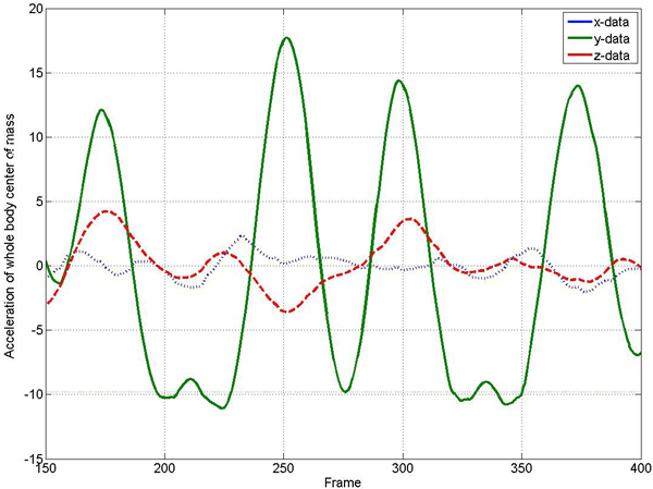
This situation is illustrated by Figure 1, which shows the COM acceleration for a dancing motion. Note that there are three flight phases, which are revealed by the vertical component (y-axis) of the COM acceleration. Further examples are discussed in Section 3.3.
Dynamic time warping (DTW) is a well-known technique to find an optimal alignment (encoded by a so-called warping path) between two given sequences. Based on the alignment, the sequences can be warped in a non-linear fashion to match each other. In our context, each motion sequence is converted into a sequence of physics-based motion features at a temporal resolution of 120 Hz. We denote by V ≔ (v1,v2,...,vn) and W ≔ (w1,w2,...,wm) the feature sequences of the two motions to be aligned. Since one of the motions might be slower than the other, n and m do not have to be equal.
In a second step, one computes an n x m cost matrix C with respect to some local cost measure c, which is used to compare two feature vectors. In our case, we use a simple cost measure, which is based on the inner product:
for two non-zero feature vectors v and w (otherwise
c(v,w) is set to zero). Note that c(v,w) is zero in case v
and w coincide and assumes values in the real interval
[0,1] ⊂
. Then, the cost matrix C with respect to the
sequences V and W is defined by
C(i,j) ≔ c(vi,wj
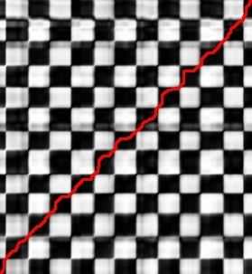
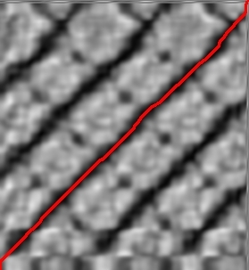
for 1 ≤ i ≤ n and 1 ≤ j ≤ m. Figure 2 shows such cost matrices with respect to different features.
Finally, an optimal alignment is determined from the cost matrix C via dynamic programming. Such an alignment is represented by a so-called (cost-minimizing) warping path, which, under certain constraints, optimally allocates the frame indices of the first motion with the frame indices of the second motion. In Figure 2, such optimal warping paths are indicated in red. Note that the information given by an optimal warping path can be used to time-warp the second motion (by suitably omitting or replicating frames) to match the first motion. Further details and references on DTW may be found in [ ZM06 ].
Note that the time and memory complexity of the DTW algorithm is quadratic in the number of frames of the motions to be aligned. To speed up the process, we employ an iterative multiscale DTW algorithm as described in [ ZM06 ]. Here, the idea is to proceed iteratively using multiple resolution levels going from coarse to fine. In each step, the warping path computed at a coarse resolution level is projected to the next higher level, where the projected path is refined to yield a warping path at the higher level. To obtain features at the coarse levels, we use simple windowing and averaging procedures. In this context, the physics-based features have turned out to yield semantically meaningful features even at a low temporal resolution. In our implementation, we used six different resolution levels starting with a feature resolution of 4 Hz at the lowest level. The overall speed-up of this approach (in comparison to classical DTW) depends on the length of the motion sequences. For example, the speed-up amounts to a factor of roughly 10 for motions having 300 frames and a factor of roughly 100 for motions having 3000 frames.
Figure 2 shows two cost matrices, where we compared two walking motions both consisting of 6 steps forward. In dark areas the compared poses are similar with respect to the given features, whereas in lighter areas the poses are dissimilar. The red line is the optimal warping path found by the DTW algorithm. The cost matrix on the left side is based only on the COM acceleration of the entire body. Using this single feature, the checkerboard-like pattern indicates that one cannot differentiate between steps that were done with the left or the right foot. Adding the features that measures the angular momenta of the feet, the result obviously improves. The resulting cost matrix is shown on the right hand side of Figure 2. The five dark diagonals indicate that in this case only the steps made with the same foot are regarded as similar.
Figure 2. DTW cost matrices calculated on the whole body COM acceleration (left) as well as on the basis of the COM acceleration and the angular momenta of the hands and feet (right). The cost-minimizing warping paths are drawn red.
Depending on the motions to be time-warped, one can select specific features. For walking motions, the movement of the legs contains the most important information in case the steps are to be synchronized.
For time-warping grabbing motions as used in our experiments, aspects concerning the right hand were most important as the motions were performed by this hand. For our cartwheel motions, good correspondences were achieved when using features that concern the two hands and the two feet. For an example of warped walking motions, we refer to the accompanying video.
For our experiments, we systematically recorded several hours of motion capture data containing a number of well-specified motion sequences, which were executed several times and performed by five different actors. The five actors all have been healthy young adult male persons. Using this data, we built up a database consisting of roughly 210 minutes of motion data. Then we manually cut out suitable motion clips and arranged them into 64 different classes and styles. Each such motion class contains 10 to 50 different realizations of the same type of motion, covering a broad spectrum of semantically meaningful variations. The resulting motion class database contains 1,457 motion clips of a total length corresponding to roughly 50 minutes of motion data [ MRC07 ]. For our experiments, we considered three motion classes. The first class contains walking motions executed in the following styles:
-
Walk four steps in a straight line.
-
Walk four steps in a half circle to the left side.
-
Walk four steps in a half circle to the right side.
-
Walk four steps on the place.
All motions within each of these styles had to start with the right foot and were aligned over time to the length of the first motion of actor one.
The second class of motions we considered in our experiments consists of various grabbing motions, where the actor had to pick an object with the right hand from a storage rack. In this example the style mode corresponds to three different heights(low, middle, and high) the object was located in the rack.
The third motion class consist of various cartwheels. Cartwheel motions were just available for four different actors and for one style. All cartwheels within the class start with the left foot and the left hand.
For all motion classes described in the previous section, we constructed data tensors with motion representations based on Euler angles and based on quaternions. Initially some preprocessing was required, consisting mainly of the following steps. All motions were
-
filtered in the quaternion domain with a smoothing filter described as in [ LS02 ],
-
normalized by moving the root nodes to the origin and by orienting the root nodes to the same direction,
In this section, we discuss various truncation experiments for our three representative example motion classes. In these experiments, we systematically truncated a growing number of components of the core-tensors, then reconstructed the motions, and compared them with the original motions.
Based on the walking motions (using quaternions to
represent the orientations), we constructed two data
tensors. The first tensor
 was constructed by
using the Data Mode as technical mode. This is indicated
by the upper index, which shows the dimension of the
tensor. The motions were time-warped and sampled
down to a length of 60 frames. The resulting size of
is 7140 x 5 x 4 x 3. Using the Frame
Mode and DOF Mode, we obtained a second tensor
was constructed by
using the Data Mode as technical mode. This is indicated
by the upper index, which shows the dimension of the
tensor. The motions were time-warped and sampled
down to a length of 60 frames. The resulting size of
is 7140 x 5 x 4 x 3. Using the Frame
Mode and DOF Mode, we obtained a second tensor
 of size 60 x 119 x 5 4 x 3. Table 1
shows the results of our truncation experiments. The first
column shows the size of the core tensors
'Walk
after
truncation, where the truncated modes are colored red.
The second column shows the number of entries of the
core tensors, and the third one shows its size in percent
compared to ΔWalk
. In the fourth column, the total
usage of memory is shown. Note that the total memory
requirements may be higher than for the original data,
since besides the core tensor
' one also has to store the
matrices U'k
. The memory requirements are particulary
high in case one mode has a high dimension. The last
two columns give the results of the reconstruction.
Etotal
is an error measurement which is defined as
the sum over the reconstruction error Emot
over all
motions:
of size 60 x 119 x 5 4 x 3. Table 1
shows the results of our truncation experiments. The first
column shows the size of the core tensors
'Walk
after
truncation, where the truncated modes are colored red.
The second column shows the number of entries of the
core tensors, and the third one shows its size in percent
compared to ΔWalk
. In the fourth column, the total
usage of memory is shown. Note that the total memory
requirements may be higher than for the original data,
since besides the core tensor
' one also has to store the
matrices U'k
. The memory requirements are particulary
high in case one mode has a high dimension. The last
two columns give the results of the reconstruction.
Etotal
is an error measurement which is defined as
the sum over the reconstruction error Emot
over all
motions:
The reconstruction error Emot of a motion is defined as normalized sum over all frames and over all joints:
where f denotes the number of frames and m the number of quaternions. Here, for each joint, the original and reconstructed quaternions qorg and qrec are compared by means of their included angle. We performed a visual rating for some of the reconstructed motions in order to obtain an idea of the quality of our error measurement. Here, a reconstructed motion was classified as good (or better) in case one could hardly differentiate it from the original motion when both of the motions were put on top of each other. The results of our ratings are given in the last column.
Table 1. Results for truncating technical and natural modes from our tensors filled with walking motions (using quaternions).
|
Dimension core tensor |
Entries core tensor |
Size core tensor in percent |
Memory usage in percent |
Etotal |
visual rating |
|
Truncation of Data Mode of
|
|||||
|
7140 x 5 x 4 x 3 |
428 400 |
100 % |
12 000 % |
0.0000 |
excellent |
|
60 x 5 x 4 x 3 |
3 600 |
0.8403 % |
100.8520 % |
0.0000 |
excellent |
|
53 x 5 x 4 x 3 |
3 180 |
0.7423 % |
89.0873 % |
0.0000 |
excellent |
|
52 x 5 x 4 x 3 |
3 120 |
0.7283 % |
87.4066 % |
0.0634 |
excellent |
|
50 x 5 x 4 x 3 |
3 000 |
0.7003 % |
84.0453 % |
0.2538 |
very good |
|
40 x 5 x 4 x 3 |
2 400 |
0.5602 % |
67.2386 % |
1.1998 |
very good |
|
30 x 5 x 4 x 3 |
1 800 |
0.4202 % |
50.4318 % |
2.1221 |
very good |
|
20 x 5 x 4 x 3 |
1 200 |
0.2801 % |
33.6251 % |
3.6258 |
good |
|
10 x 5 x 4 x 3 |
600 |
0.1401 % |
16.8184 % |
6.3961 |
good |
|
5 x 5 x 4 x 3 |
300 |
0.0700 % |
8.4150 % |
9.3932 |
satisfying |
|
4 x 5 x 4 x 3 |
240 |
0.0560 % |
6.7344 % |
10.4260 |
satisfying |
|
3 x 5 x 4 x 3 |
180 |
0.0420 % |
5.0537 % |
10.9443 |
sufficient |
|
2 x 5 x 4 x 3 |
120 |
0.0280 % |
3.3730 % |
11.5397 |
poor |
|
1 x 5 x 4 x 3 |
60 |
0.0140 % |
1.6923 % |
11.8353 |
poor |
|
Truncation of Actor Mode of
|
|||||
|
60 x 4 x 4 x 3 |
2 880 |
0.6723 % |
100.6828 % |
4.3863 |
satisfying |
|
60 x 3 x 4 x 3 |
2 160 |
0.5042 % |
100.5135 % |
6.4469 |
satisfying |
|
60 x 2 x 4 x 3 |
1 440 |
0.3361 % |
100.3443 % |
8.2369 |
satisfying |
|
60 x 1 x 4 x 3 |
720 |
0.1681 % |
100.1751 % |
10.7773 |
sufficient |
|
Truncation of Style Mode of
|
|||||
|
60 x 5 x 3 x 3 |
2 700 |
0.6303 % |
100.6410 % |
3.5868 |
good |
|
60 x 5 x 2 x 3 |
1 800 |
0.4202 % |
100.4300 % |
5.8414 |
sufficient |
|
60 x 5 x 1 x 3 |
900 |
0.2101 % |
100.2190 % |
8.5770 |
poor |
|
Truncation of Repetition Mode of
|
|||||
|
60 x 5 x 4 x 2 |
285 600 |
66,667 % |
100.5712 % |
2.7639 |
good |
|
60 x 5 x 4 x 1 |
142 800 |
33,333 % |
100.2904 % |
5.0000 |
good |
|
Truncation of Frame and DOF Mode of
|
|||||
|
26 x 91 x 5 x 4 x 3 |
141960 |
20.9288 % |
22.8968 % |
0.5492 |
very good |
|
21 x 91 x 5 x 4 x 3 |
114660 |
16.9040 % |
18.8020 % |
0.7418 |
very good |
|
21 x 46 x 5 x 4 x 3 |
57960 |
8.5449 % |
9.6534 % |
0.9771 |
very good |
|
15 x 34 x 5 x 4 x 3 |
30 600 |
4.5113 % |
5.3252 % |
1.9478 |
good |
|
14 x 35 x 5 x 4 x 3 |
29 400 |
4.3344 % |
5.1519 % |
1.9817 |
good |
|
13 x 37 x 5 x 4 x 3 |
28 860 |
4.2548 % |
5.0933 % |
1.9724 |
good |
|
12 x 39 x 5 x 4 x 3 |
28 800 |
4.1398 % |
4.9994 % |
1.9907 |
good |
If the Data Mode is split up into the Frame and DOF
Mode, as in
, one can truncate the two modes
separately. The results are shown in the lower part of
Table 1 and Figure 3.
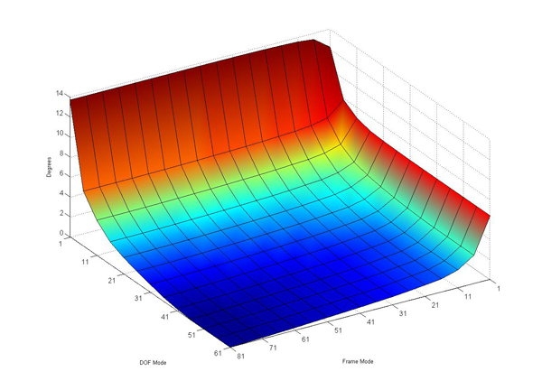
For example, reducing the DOF Mode from 60 to 26, the error Etotal is still less than one degree. A similar result is reached by reducing the Frame Mode down to a size of 20. This shows that there is a high redundancy in the data with respect to the technical modes.
We also conducted experiments, where we reduced the dimensions of the natural modes. As the experiments suggest, the dimensions of the natural modes seem to be more important than the ones of the technical modes. The smallest errors (when truncating natural modes) resulted by truncating the Repetition Mode. This is not surprising since the actors were asked to perform the same motion several times in the same fashion. Note that different interpretations by one and the same actor reveal a smaller variance than motions performed by different actors or motions performed in different styles. Some results of our experiments are illustrated by Figure 4.
Figure 4. Error Etotal , of reconstructed motions where two natural Modes were truncated. Actor and Style Mode are truncated (left). Actor and Repetition Mode are truncated (middle). Style and Repetition Mode are truncated (right).
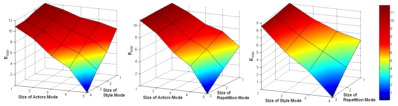
The displacement grows with the size of truncated values from Style- and Personal Mode.
For building the data tensors
 and
and
 , all motions were warped to the length
of one reference motion.
has a size of
8449 x 5 x 3 x 3, while
has a size of
71 x 119 x 5 x 3 x 3. The exact values for truncating the
Data Mode and the DOF Mode can be found in Table
2.
, all motions were warped to the length
of one reference motion.
has a size of
8449 x 5 x 3 x 3, while
has a size of
71 x 119 x 5 x 3 x 3. The exact values for truncating the
Data Mode and the DOF Mode can be found in Table
2.
Table 2. Truncation results for grabbing motions (using quaternions).
|
Dimension core tensor |
Entries core tensor |
Size core tensor in percent |
Memory usage |
Etotal |
visual rating in percent |
|
Truncation of Data Mode of
|
|||||
|
8449 x 5 x 3 x 3 |
380 205 |
100 % |
18 775 % |
0.0000 |
excellent |
|
60 x 5 x 3 x 3 |
2 700 |
0.7101 % |
134.0548 % |
0.0000 |
excellent |
|
55 x 5 x 3 x 3 |
2 475 |
0.6510 % |
122.8845 % |
0.0000 |
excellent |
|
50 x 5 x 3 x 3 |
2 250 |
0.5918 % |
111.7142 % |
0.0000 |
excellent |
|
45 x 5 x 3 x 3 |
2 025 |
0.5326 % |
100.5439 % |
0.0000 |
excellent |
|
40 x 5 x 3 x 3 |
1 800 |
0.4734 % |
89.3736 % |
1.2632 |
very good |
|
35 x 5 x 3 x 3 |
1 575 |
0.4143 % |
78.2033 % |
2.1265 |
very good |
|
30 x 5 x 3 x 3 |
1 350 |
0.3551 % |
67.0330 % |
2.9843 |
very good |
|
25 x 5 x 3 x 3 |
1 125 |
0.2959 % |
55.8628 % |
3.9548 |
good |
|
20 x 5 x 3 x 3 |
900 |
0.2367 % |
44.6925 % |
5.1628 |
good |
|
15 x 5 x 3 x 3 |
675 |
0.1775 % |
33.5222 % |
6.6799 |
satisfying |
|
10 x 5 x 3 x 3 |
450 |
0.1184 % |
22.3519 % |
8.8702 |
sufficient |
|
5 x 5 x 3 x 3 |
225 |
0.0592 % |
11.1816 % |
11.5604 |
sufficient |
|
4 x 5 x 3 x 3 |
180 |
0.0473 % |
8.9475 % |
12.4463 |
poor |
|
3 x 5 x 3 x 3 |
135 |
0.0355 % |
6.7135 % |
12.7304 |
poor |
|
2 x 5 x 3 x 3 |
90 |
0.0237 % |
4.4794 % |
13.4234 |
poor |
|
1 x 5 x 3 x 3 |
45 |
0.0118 % |
2.2454 % |
13.7150 |
poor |
|
Truncation of DOF Mode of
|
|||||
|
71 x 91 x 5 x 3 x 3 |
290 745 |
76.4706 % |
80.6560 % |
0.0000 |
excellent |
|
71 x 86 x 5 x 3 x 3 |
274 770 |
72.2689 % |
76.2978 % |
0.0001 |
excellent |
|
71 x 61 x 5 x 3 x 3 |
194 895 |
51.2605 % |
54.5069 % |
0.1311 |
excellent |
|
71 x 51 x 5 x 3 x 3 |
162 945 |
42.8571 % |
45.7906 % |
0.4332 |
good |
|
71 x 41 x 5 x 3 x 3 |
130 995 |
34.4538 % |
37.0742 % |
1.0450 |
satisfying |
|
71 x 31 x 5 x 3 x 3 |
99 045 |
26.0504 % |
28.3579 % |
2.2182 |
sufficient |
|
71 x 21 x 5 x 3 x 3 |
67 095 |
17.6471 % |
19.6415 % |
3.9491 |
sufficient |
|
71 x 11 x 5 x 3 x 3 |
35 145 |
9.2437 % |
10.9252 % |
7.1531 |
poor |
|
71 x 6 x 5 x 3 x 3 |
19 170 |
5.0420 % |
6.5670 % |
10.1546 |
poor |
|
71 x 1 x 5 x 3 x 3 |
3 195 |
0.8403 % |
2.2088 % |
14.3765 |
poor |
In our third example, we consider a motion class
consisting of cartwheel motions. The core tensor
 has a size of 7497 x 4 x 1 x 3. Here, all
motions could be reconstructed without any visible
error for a size of no more than 12 dimensions for
the Data Mode. Further results are shown in Table
3.
has a size of 7497 x 4 x 1 x 3. Here, all
motions could be reconstructed without any visible
error for a size of no more than 12 dimensions for
the Data Mode. Further results are shown in Table
3.
Table 3. Truncation results for cartwheel motions (using quaternions).
|
Dimension core tensor |
Entries core tensor |
Size core tensor in percent |
Memory usage |
Etotal |
visual rating in percent |
|
Truncation of Data Mode of
|
|||||
|
30 x 4 x 3 |
360 |
0.4002 % |
250.4279 % |
0.0000 |
excellent |
|
12 x 4 x 3 |
144 |
0.1601 % |
100.1879 % |
0.0000 |
excellent |
|
11 x 4 x 3 |
132 |
0.1467 % |
91.8412 % |
1.6780 |
good |
|
10 x 4 x 3 |
120 |
0.1334 % |
83.4945 % |
3.2163 |
satisfying |
|
9 x 4 x 3 |
108 |
0.1200 % |
75.1478 % |
5.7641 |
sufficient |
|
8 x 4 x 3 |
96 |
0.1067 % |
66.8012 % |
8.1549 |
poor |
|
5 x 4 x 3 |
60 |
0.0667 % |
41.7611 % |
13.2847 |
poor |
|
1 x 4 x 3 |
12 |
0.0133 % |
8.3745 % |
22.4095 |
poor |
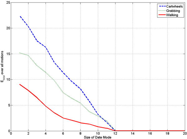
The number of necessary components of the data mode
varied a lot in the different motion classes. One would
expect that a cartwheel motion is more complex than a
grabbing or walking motion. The results of previous
experiments do not support this prospect. But the results
of this truncation experiments are not comparable as they
depend on all dimensions of the constructed tensors. To
get comparable results for the three motion classes, we
constructed a tensor including three motions from three
actors for each motion class. The style mode is limited to a
size of one, since we have no different styles for cartwheel
motions. Therefor the resulting tenors have a size of
f ⋅ n x 3 x 3 x 1. When truncating the data mode
of these tensors, one gets the result that is shown in
Figure 5. All motions are reconstructed perfectly until
the size of the data mode gets smaller than 12. At
this size the core tensor
' and the matrices Uk
have
as many entries as the original data tensor Δ. Then
the error Etotal
grows different for the three motion
classes. The smallest error is observed for the walking
motions (solid). This could be expected for a cyclic
motion that contains a lot of redundant frames. The used
grabbing motions (dotted) are more complex. The reason
may be that the motions sequences disparate since
some sequences include a step to the storage rack
while others do not. The cartwheel motions (dashed)
are the most complex class in this experiment, as we
expected.
Figure 5. Reconstruction error Etotal for walking (solid), grabbing (dotted) and cartwheel (dashed) motions, depending on the size of the Data Mode of the core tensor.
To compare our multilinear model with linear models, as they are used for principal component analysis (PCA), we constructed two tensors for our model and two matrices for the PCA. The first tensor and the first matrix were filled with walking motions, the second tensor and the second matrix were filled with grabbing motions. The orientations were represented by Euler angles. The resulting tensors had a size of 81 x 62 x 3 x 3 x 3 (walking) and 64 x 62 x 3 x 3 x 3 (grabbing), respectively.
Figure 6. Mean error of reconstructed motions with reconstructions based on our model (blue) and based on a PCA (green). The result is shown for walking motions (left) and grabbing motions (right).
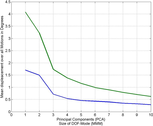
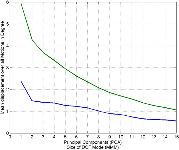
After some data reduction step, we compared the reconstructed motions with the original motions by measuring the differences between all orientations of the original and the reconstructed motions. Averaging over all motions and differences, we obtained a mean error as is also used in [ SHP04 ] (we used this measure to keep the results comparable to the literature). Figure 6 shows a comparison of the mean errors in the reconstructed motions for the walking (left) and grabbing (right) examples. The mean errors depend on the size of the DOF Mode and the number of principal components, respectively. Note that the errors for motions reconstructed from the multi-mode-model are smaller than the errors from the motions reconstructed from principal components. For example, a walking motion can be reconstructed with a mean error of less than one degree (in the average) from a core tensor when the DOF Mode is truncated to just three components (see left part of Figure 6). Therefore, in cases where a motion should be approximated by rather few components the reduction based on the multilinear model may be considerably better than the one achieved by PCA.
As it was described in Sect. 2.3, it is possible to
synthesize motions with our multilinear model. For every
mode k there is an appropriate matrix Uk
, where every
row uk,j
with j ∈ {1,2,...,dk} represents one of
the dimensions, of mode k. Therefore an inter- or
extrapolation between the dk
dimensions e.g. between the
styles, actors and repetitions, can be done by inter- or
extrapolation between any rows of Uk
before they are
multiplied with the core tensor
to synthesize a motion.
To prevent our results from artifacts such as turns and
unexpected flips resulting from a representation based on
Euler angles we used our quaternion based representation
to synthesize motions.
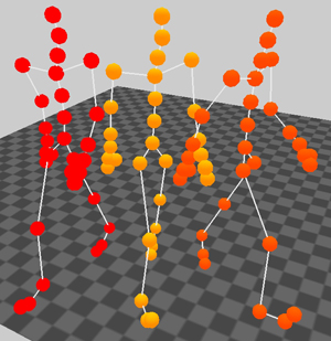
For the following walking example, we constructed a motion that was interpolated between two different styles. The first style was walking four steps straight forward and the second one was walking four steps on a left circle. We made a linear interpolation by multiplying the corresponding rows with the factor 0.5. The result is a four step walking motion that describes a left round with a larger radius. One sample frame of this experiment can be seen in Figure 7. Another synthetic motion was made by an interpolation of grabbing styles.
Figure 7. Screenshot from the original motions that are from the styles walking forward (left) and walking a left circle (right), the synthetic motion (middle) is produced by a linear combination of these styles.
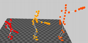
We synthesized a motion by an interpolation of the styles grabbing low and grabbing high. The result is a motion that grabs in the middle. One sample frame of this synthetic motion is shown in Figure 8.
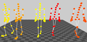
With this technique we are able to make interpolation between all modes simultaneous. One example is a walking motion that is an interpolation between the Style and Actors Mode. One snapshot taken from the accompanying animation video of this example is given in Figure 8.
Figure 8. Left: Screenshot from the original motions that are from the styles grabbing low (left) and grabbing high (right), the synthetic motion (middle) is produced by a linear combination of these styles. Right: Screenshot from four original walking motions and one synthetic motion, that is an result of combining two, the personal and the style mode. The original motions of the first actor are on the left side, the original motions of the second actor are on the right side and the synthetic example can be seen in the middle.
In Table 4 the computation times of our MATLAB
implementations of the N-Mode SVD and PCA are
given (on an 1.66 GHz Intel Core2 CPU T5500).
For the decomposition of a data tensor
consisting of 95 x 119 x 4 x 3 x 2 = 273600 entries, the
N-Mode SVD needs 5.675 seconds, while the PCA needs
0.636 seconds for a matrix of comparable size having
119 x 2280 = 273600 entries. As Table 4 shows, the
computing time for the SVD increase with the dimension
of the tensor, while the computation time for the PCA is
nearly constant.
The SVD decomposition can be seen as a preprocessing
step, where all further calculations can be done on
the core tensor and the corresponding matrices. The
reconstruction of a motion from the tensor
 and the matrices Uk
can be performed at interactive
frame rates—even in our MATLAB implementation
the reconstruction only requires 0.172 seconds. As a
combination of motions of different modes is just a
reconstruction with modified weights, the creation
of synthetic motions is also possible with a similar
computational cost.
and the matrices Uk
can be performed at interactive
frame rates—even in our MATLAB implementation
the reconstruction only requires 0.172 seconds. As a
combination of motions of different modes is just a
reconstruction with modified weights, the creation
of synthetic motions is also possible with a similar
computational cost.
Table 4. Computation times for PCA and N-Mode-SVD for the data used in the examples.
|
Dimension Motion Matrix |
Time PCA (in sec.) |
Dimension Core Tensor |
Time N-Mode SVD (in sec.) |
|
119 x 2280 |
0.636 |
95 x 119 x 4 x 3 x 2 |
5.675 |
|
95 x 2280 |
0.621 |
95 x 95 x 4 x 3 x 2 |
4.968 |
|
80 x 2280 |
0.615 |
95 x 80 x 4 x 3 x 2 |
4.461 |
|
5 x 2280 |
0.600 |
95 x 5 x 4 x 3 x 2 |
2.295 |
In this paper, we have shown how multilinear models can be used for analyzing and processing human motion data. The representation is based on explicitly using various modes that correspond to technical as well as semantic aspects of some given motion class. Encoding the data as high-order tensors allows for reducing the model with respect to any combination of modes, which often yields better approximation results than previously used PCA-based methods. Furthermore, the multilinear model constitutes a unified and flexible framework for motion synthesis applications, which allows for controlling each motion aspect independently in the morphing process. As a further contribution, we described an efficient multiscale approach for motion warping using physics-based motion features.
Multilinear motion representations constitute an interesting alternative and additional tool in basically all situations, where current PCA-based methods are used. We expect that our multi-modal model is helpful in the context of reconstructing motions from low-dimensional control signals, see, e. g., [ CH05 ]. Currently, we also investigate how one can improve auditory representations of motions as described in [ RM05, EMWZ05 ] by using strongly reduced motion representations.
In order to construct a high-order tensor for a given motion class, one needs a sufficient number of example motions for each mode to be considered in the model. In practice, this is often problematic, since one may only have sparsely given data for the different modes. In suchsituations, one may employ similar techniques as have been employed in the context of face transfer, see [ VBPP05 ], to fill up the data tensor. Another important research problem concerns the automatic extraction of suitable example motions from a large database, which consists of unknown and unorganized motion material. For the future, we plan to employ efficient content-based motion retrieval strategies as described, e. g., in [ KG04, MRC05, MR06 ] to support the automatic generation of multimodal data tensors for motion classes that have a sufficient number of instances in the unstructured dataset.
We are grateful to Bernd Eberhardt and his group from HDM Stuttgart for providing us with the mocap data. We also thank the anonymous referees for constructive and valuable comments.
[BA00] The N-way Toolbox for MATLAB, 2000, http://www.models.kvl.dk/source/nwaytoolbox/, last visited June 10th, 2008.
[BSP04] Segmenting motion capture data into distinct behaviors, Proceedings of the Graphics Interface 2004 Conference, Wolfgang Heidrich and Ravin Balakrishnan (Eds.), pp. 185—194, Canadian Human-Computer Communications Society, London, Ontario, Canada, 2004, isbn 1-56881-227-2.
[BW95] Motion signal processing, Proceedings of the 22nd annual conference on Computer graphics and interactive techniques, Robert Cook (Ed.), ACM Press, New York, 1995, pp. 97—104, isbn 0-80791-701-4.
[CH05] Performance animation from low-dimensional control signals, ACM Trans. Graph., (2005), no. 3, SIGGRAPH 2005, 686—696, issn 0730-0301.
[CH07] Constraint-based Motion Optimization Using A Statistical Dynamic Model, ACM Transactions on Graphics, (2007), no. 3, Article no. 8, SIGGRAPH 2007, issn 0730-0301.
[EMWZ05] MotionLab Sonify: A Framework for the Sonification of Human Motion Data, Ninth International Conference on Information Visualisation (IV'05), July 2005, IEEE Press, London, UK, pp. 17—23, isbn 0-7695-2397-8.
[FF05] An efficient search algorithm for motion data using weighted PCA, Proc. 2005 ACM SIGGRAPH/Eurographics Symposium on Computer Animation, 2005, ACM Press, Los Angeles, California, pp. 67—76, isbn 1-7695-2270-X.
[GBT04] PCA-Based Walking Engine Using Motion Capture Data, CGI '04: Proceedings of the Computer Graphics International (CGI'04), IEEE Computer Society, Washington, DC, USA, 2004, pp. 292—298, isbn 0-7695-2171-1.
[GP00] Morphable Models for the Analysis and Synthesis of Complex Motion Patterns, International Journal of Computer Vision, (2000) , no. 1, pp. 59—73 issn 0920-5691.
[HPP05] Style translation for human motion, ACM Trans. Graph., (2005), no. 3, 1082—1089, issn 0730-0301.
[KG03] Flexible Automatic Motion Blending with Registration Curves, Eurographics/SIGGRAPH Symposium on Computer Animation, D. Breen and M. Lin (Eds.), San Diego, California, Eurographics Association, 2003, pp. 214—224, isbn 1-58113-659-5.
[KB04] Automated extraction and parameterization of motions in large data sets, ACM Transactions on Graphics, (2004), no. 3, SIGGRAPH 2004, 559—568, issn 0730-0301.
[KGP02] Motion Graphs, ACM Transactions on Graphics, (2002), no. 3, SIGGRAPH 2002, 473—482, issn 0730-0301.
[LS02] General Construction of Time-Domain Filters for Orientation Data, IEEE Transactions on Visualizatiuon and Computer Graphics, (2002), no. 2, 119—128, issn 1077-2626.
[LZWM05] A system for analyzing and indexing human-motion databases, Proc. 2005 ACM SIGMOD Intl. Conf. on Management of Data, ACM Press, Baltimore, Maryland, 2005, pp. 924—926, isbn 1-59593-060-4.
[MK06] Multilinear Motion Synthesis Using Geostatistics, ACM SIGGRAPH / Eurographics Symposium on Computer Animation - Posters and Demos, 2006, pp. 21—22.
[MR06] Motion Templates for Automatic Classification and Retrieval of Motion Capture Data, SCA '06: Proceedings of the 2006 ACM SIGGRAPH/Eurographics Symposium on Computer Animation, ACM Press, Vienna, Austria, 2006, pp. 137—146, isbn 3-905673-34-7.
[MRC05] Efficient content-based retrieval of motion capture data, ACM Trans. Graph., (2005), no. 3, SIGGRAPH 2005, 677—685, issn 0730-0301.
[MRC07] Documentation: Mocap Database HDM05, CG-2007-2, Computer Graphics Technical Report, Universität Bonn, 2007, issn 1610-8892.
[MZF06] Automatic Splicing for Hand and Body Animations, ACM SIGGRAPH / Eurographics Symposium on Computer Animation, 2006, pp. 309—316, isbn 3-905673-34-7.
[OBHK05] Representing cyclic human motion using functional analysis, Image Vision Comput., (2005), no. 14, 1264—1276, issn 0262-8856.
[RCO05] D-12-79 A Study of Synthesizing New Human Motions from Sampled Motions Using Tensor Decomposition, Proceedings of the IEICE General Conference, The Institute of Electronics, Information and Communication Engineers, 2005, , no. 2, p. 229.
[RM05] Playing Audio-only Games: A compendium of interacting with virtual, auditory Worlds, Proceedings of Digital Games Research Conference, 2005, Vancouver, Canada.
[RW03] Development of a Computer Tool for Anthropometric Analyses, Proceedings of the International Conference on Mathematics and Engineering Techniques in Medicine and Biological Sciences (METMBS'03), CSREA Press, Las Vegas, USA, June 2003, Faramarz Valafar and Homayoun Valafar (Eds.), pp. 347—353, isbn 1-932415-04-1.
[SH05] Analyzing the physical correctness of interpolated human motion, SCA '05: Proceedings of the 2005 ACM SIGGRAPH/Eurographics symposium on Computer animation, ACM Press, New York, NY, USA, 2005, Demetri Terzopoulos ans Victor Zordan (Eds.), pp. 171—180, isbn 1-59593-198-8.
[SH07] Construction and Optimal Search of Interpolated Motion Graphs, ACM Transactions on Graphics (2007), no. 3, SIGGRAPH 2007, issn 0730-0301.
[SHP04] Synthesizing physically realistic human motion in low-dimensional, behavior-specific spaces, ACM Transactions on Graphics, (2004), no. 3, SIGGRAPH 2004, 514—521, issn 0730-0301.
[Tro02] Decomposing biological motion: A framework for analysis and synthesis of human gait patterns, , Journal of Vision, (2002), no. 5, 371—387, issn 1534-7362.
[Vas02] Human motion signatures: Analysis, synthesis, recognition, Proc. Int. Conf. on Pattern Recognition, , 2002, Quebec City, Canada, pp. 456—460, isbn 0-7695-1695-X.
[VBPP05] Face transfer with multilinear models, ACM Trans. Graph., (2005), no. 3, SIGGRAPH 2005, 426—433, issn 0730-0301.
[ZM06] Technical Report, CG-2006-1, Universität Bonn, 2006, http://cg.cs.uni-bonn.de/publications/publication.asp?id=283, Last visited June 12th, 2008, issn 1610-8892.
Additional Material
Video
| Tensor_Representation.avi | |
| Type | Video |
| Filesize | 8,6Mb |
| Length | 3:18 min |
| Language | - |
| Videocodec | DivX5.0 |
| Audiocodec | - |
| Resolution | 720x480 |
Morphing of motion by interpolation of two different styles (Walking,Grabbing). Examples for motion reconstruction. Motion Preprocessing. Time Warping Example. Examples for extreme style interpolation. |
|
| Tensor Representation | |
Volltext 
-
 Volltext als PDF
(
Größe:
2.0 MB
)
Volltext als PDF
(
Größe:
2.0 MB
)
Lizenz 
Jedermann darf dieses Werk unter den Bedingungen der Digital Peer Publishing Lizenz elektronisch übermitteln und zum Download bereitstellen. Der Lizenztext ist im Internet unter der Adresse http://www.dipp.nrw.de/lizenzen/dppl/dppl/DPPL_v2_de_06-2004.html abrufbar.
Empfohlene Zitierweise 
Björn Krüger, Jochen Tautges, Meinard Müller, and Andreas Weber, Multi-Mode Tensor Representation of Motion Data. JVRB - Journal of Virtual Reality and Broadcasting, 5(2008), no. 5. (urn:nbn:de:0009-6-14197)
Bitte geben Sie beim Zitieren dieses Artikels die exakte URL und das Datum Ihres letzten Besuchs bei dieser Online-Adresse an.
-
 News
News