Digitizing human motion has become a very important task in many VR-based applications. Besides tracking single limbs, e.g. for head tracking, one is especially interested in capturing full body setups. This is not only needed for the visualization of an actor's interaction witha scene, but also enables the generation of realistic movements for virtual characters with different properties, such as different limb lengths or muscle force (retargeting). Motion data can furthermore be used to identify and resolve faulty poses by investigation of previously generated motion statistics. For motion analysis, the data can be analyzed to deduce normal and pathological movement patterns, for example. The latter is often done in medicine and sport science, and requires accurately captured movements of the patients.

A common technique to acquire basic motion data in these applications is to use optical motion tracking systems [ Adv , Vic ] to reconstruct the 3D trajectories of special markers. With the markers attached to key positions of the actor's body, the resulting data can be used by special capturing applications to map the movements of the actor onto a virtual model.

Many such applications exist, but most of them either assume a certain recording setup and/or demand high time requirements for the session preparations, i.e. for mounting a set of special markers at pre-defined positions on each limb. These factors seriously complicate the recording process and limit the usability of such approaches in motion capture related application areas, especially in highly dynamic VR environments with possibly many different subjects. Here, an automatic and ad hoc configurable method would be very desirable.

In previous work, we presented a flexible motion tracking pipeline [ HSK05 ], which allows the computation of coordinate systems for arbitrarily placed marker bodies and the extraction of the actor's skeletal topology and geometry in a highly automated fashion. However, the resulting coordinate systems depend on the recording setup and are not aligned to the skeleton structure. Due to this fact, applications utilizing the coordinate systems, such as retargeting, involve extra pre-processing. It is also hard to reproduce or compare experiments since they have no common data basis. A further restriction of the method is that no motion parameterization is computed, which complicates post-processing and retargeting of the data.

The main contribution of this paper is to solve the above problems by extending our previous work [ HSK05 ] with two additional processing stages. The first stage normalizes the motion data to a recording-independent and common data basis, while the second stage computes a minimal and intuitive parameterization of the motion sequence. The only additional requirement is a short calibration phase in which the actor moves his limbs along main movement axes.

In the context of motion tracking and simulation, creating a common, normalized basis for character representation is normally addressed by pre-specified and standardized models [ Hum , Cen ] or strict guidelines for the motion recording setup.

In biomedical applications, such as gait analysis, typically a lot of time is invested in accurately placing the marker bodies [ SDSR99 , BBH03 ]. While these tedious preparations do create a common data basis up to a certain level, the approach is limited to a specific recording setup, and comparable only between persons with similar shape.

[ HFP00 , RL02 , Dor03 ] reduce the number of required markers by placing only few markers at specific locations on the body. The mapping between markers and body positions is then computed using a pre-specified skeleton model. [ CH05 ] use a motion database to compensate for missing skeleton parameters instead. As these methods must be adjusted to a given setup and/or actors, they are not suited for dynamic VR environments requiring flexible setups.

Specifications for limb coordinate systems were published by [ HSLC99 ] based on the anatomical planes of the body (see, for example, [ NP03 ]). These planes are based on the skeleton structure, which is independent of the recording setup. Our approach extends this work by relating the anatomical planes to the joint distribution of the body.

For the parameterization of motion data, a common approach is to parameterize a pose by specifying the position of each limb w.r.t. the joint to which it is attached.

A widely accepted parameterization technique are Euler angles, and, very similar to that approach, the JCS-method, which essentially differs in choosing the corresponding coordinate system axes aligned to the incident limbs [ GS83 ]. Both representations lack minimality since they use three angles even for joints having fewer degrees of freedom. Furthermore, these approaches are quite unintuitive in their use and suffer from the gimbal lock singularity.

[ Kea05 ] use an approach in which the axes are defined based on the body planes, and angles are measured between the current and the default position of the attached limb [ NP03 ]. This approach is based on the moving abilities of the body, and leads to a minimal set of parameters per limb. However, the anatomical axes do not always coincide with the actual movement axes [ Bak03 , WHV05 ].

Our work addresses the above mentioned problems by dynamically extracting the movement axes corresponding to the degrees of freedom described in [ Kea05 ] from a calibration phase performed during the recording session and a subsequent automatic parameterization phase.

Figure 1.  Skeleton Normalization. (a) Recording setup. (b) Motion captured raw data based on (a). The marker bodies are recording-dependent. (c) Default position and body planes. (d) The normalized coordinate systems are aligned to the skeleton structure.

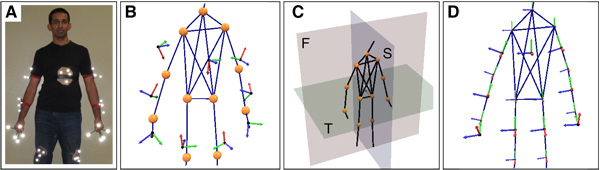
Focussing on highly dynamic VR environments, we showed in [ HSK05 ] how to extract coordinate systems for marker bodies arbitrarily placed on the limbs and to automatically reconstruct the skeletal topology (Fig. 1b ). However, as outlined in the previous sections, VR applications for motion data acquisition and retargeting, could be greatly simplified if the coordinate systems were aligned to the skeleton structure. In this section we describe how such a normalization can be achieved for arbitrary recording setups. Please refer to [ Sar05 ] for a more detailed description.

The normalization stage extracts the recording independent body planes based on the available skeletal geometry and uses them to recompute the coordinate systems aligned to the skeleton. The body planes are based on the so called default position of the body [ HSLC99 , NP03 ], illustrated in Fig. 1 c. This figure also shows the three body planes: the frontal plane separates front and back, the sagittal plane left and right, and the transverse plane top and bottom of the body.

We require an approximate default position to appear in at least one frame of the recorded motion data. The frame representing the default position best is identified by associating a cost value with each frame, which captures the essential characteristics of the default position based on heuristics of the joint positions: the average squared distance to their best fitting plane, the edge ratio of the 2D bounding box of the joints projected into that plane, and the average distance of the joints to their center of gravity [ Sar05 ]. In our experiments this technique succeeded in reliably finding the frame containing the best candidate for the default position. Based on this frame, the frontal plane is the best fitting plane through the joints, the transverse plane is chosen orthogonally such that the angle between its normal and the global up-direction is minimized, and the sagittal plane is orthogonal to both other planes. The body planes' normals yield the body coordinate system.

The re-computation of the normalized coordinate systems for every limb in the default position frame works by first assigning the body coordinate system to the torso as the hierarchical root of the skeleton structure. Then, we compute for each limb its main orientation by analyzing the neighboring joints. We select the two body plane normals which span the smallest angle with the plane orthogonal to the main orientation. Projecting these normals into the plane yields, together with the axis along the main orientation, an orthogonal coordinate system for the limb, which is placed in its mid point.

Based on the original and normalized coordinate systems for the default position we can propagate the corresponding transformations to all frames, yielding consistently oriented coordinate systems for the whole recording aligned with the skeleton structure (Fig. 1d).

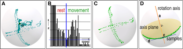
Figure 2. Skeleton Parameterization. (a) Illustration of limb positions. (b) Histogram of movement speeds. (c) Samples (based on a) classified as movement samples. (d) Relation between main direction and corresponding rotation axis.

The parameterization stage described in this section computes the motion description reflecting the actual degrees of freedom at each joint of the body. Doing so yields a compact and intuitive representation, which can, for example, be used to identify tracking errors (by investigating the probability of parameter combinations) and to simplify pose editing.

In a more general approach than [ Kea05 ] we do not assume certain fixed axes, but instead dynamically extract joint axes based on the observed movements of the attached limb. For this to work, the actor is required to subsequently perform specific main movements with his or her limbs in a short calibration phase. Exerting all of the joints' degrees of freedom, these movements should represent intuitive moving directions of the individual limbs. Depending on the type of the parent joint, one or two such movements can be identified per limb [ Sar05 ]. For the upper arm, for example, this could be swinging back and forth and lifting sideways, while the forearm could be flexed and extended.

Based on the information gathered in this phase it is possible to derive an intuitive movement parameterization. First, the samples recorded during the calibration phase are classified into movement and stationary phases (filtering). The movement samples are then used to infer the axes corresponding to the main movements (axis extraction). After the start position for the rotations has been identified (rest position), the angles about the extracted axes leading to the recorded limb positions in the original data can be calculated (angle computation).

Our algorithms are based on the relative positions of the attached limb w.r.t. the parent's joint coordinate system, which is the coordinate system of the hierarchically higher limb translated to the joint center. A limb position in frame i will be called sample and denoted with p_i and S = [p₀, p₁, ..., p_n] ⊆ R³ is the set containing all samples. Note that the samples lie on a sphere around the joint center (the joint sphere, cf. Fig. 2a).

4.2. Extraction of the Movement Axes

In this subsection we describe how to extract the movement axes given the movement samples M. A first observation is that it is sufficient to extract the main direction found in the distribution, consisting of a center c and direction d along which the samples of one moving direction are oriented. The axis corresponding to this main direction is then orthogonal to the axis plane spanned by d,c, and the joint center o: a = (c − o) × d (Fig. 2c).

The problem is to automatically extract the main directions from the sample distribution. Here we will discuss the problem of two main directions (Fig. 2a) corresponding to two different rotation axes. The solution for one main direction is a straightforward regression problem.

A commonly used method to extract directions of maximal variance within a point cloud is the Principal Component Analysis (PCA, [ Smi02 ]). Since this algorithm requires a uniform sample density to produce useful results, we stratify the samples by choosing one representative each for a set of cells approximately uniformly partitioning the joint sphere.

Figure 3. Axis Extraction. The lines in a and d show the intersection of the axis planes with the sphere tangent plane which is orthogonal to both axis planes. (a) A case where both PCA and EM fail. Note that one of the planes could only be aligned badly with the corresponding samples. (b) Measuring the similarity of directions. (c) Initial direction groups (based on a). (d) Resulting axis planes. Note that the axes are much better aligned with the samples.

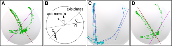
Unfortunately, the PCA results do often fail to compute proper main directions. One reason for this fact is that the PCA finds the globally optimal directions of maximal variance, which do not necessarily correspond to the desired main movement directions. Another reason is that the PCA axes are orthogonal to one another, which does not necessarily hold for the movement axes [ Bak03 , WHV05 ].

We optimized the PCA results by applying a subsequent optimization process based on Expectation Maximization (EM, [ FP02 ]). EM tries to iteratively optimize the result by an alternating repartitioning of the samples to the respective closest axis plane, and then computing new axis planes based on the updated partitions. By doing so, one can generally recover the actual main directions much better. However, for noisy data EM tends to get stuck in local optima, depending on the starting configuration (Fig. 3a).

Due to these problems, standard extraction methods are not suitable for an automatic and reliable extraction of the movement axes, and hence we developed a new method (Direction Joining) as described in the following section.

Direction Joining

Our Direction Joining algorithm exploits the sequential ordering of motion samples in the given data. It identifies consecutive samples oriented along the same direction, and then joins similarly oriented sample sets into main directions. Since a simple global stratification as used for the PCA and EM approach destroys the temporal order among the samples, we use a windowed stratification. Here, a representative is chosen for all consecutive samples falling into the same cell, i.e., there may be several representatives for a given cell.

In an initial step, consecutive samples which are oriented approximately along the same direction are grouped together. We start with a group containing the first two samples p₀ and p₁. For each group G_j we maintain its center c_j and direction d_j ; for the initial group G₀ this would be d₀ = p₁ − p₀ and c₀ = p₀ + 0.5·d₀.

Now we traverse all samples p_i(1 ≤ i ≤ n). In each step we compute the current movement vector v_i = p_i − p_i−1. If the angle between v_i and the current group's direction d_j exceeds a certain threshold δ, a new group G_j+1 is created (based on G_j+1 and p_i-1 as described above). Otherwise, p_i is added to the group, and both direction and center are updated:

  and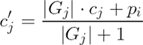  

Figure 4. Parameterization Steps. (a) The rest position being the sample closest to the intersection of the axis planes and the joint sphere. (b) Computation of the rotation angle for a single axis. (c) Computation of the rotation angles for two axes by reduction to circle intersection. (d) Twist angle computation.

Computing the angles directly between movement vectors leads to wrong results, since the samples are located on the joint sphere, and the sphere's curvature introduces an angle itself. Instead we compute the angle between the corresponding axis planes ∠(d,c,d_j,c_j) := ∠(d ×(c−o),d_j×(c_j−o)) where d = p_i−p_i−1 and c = p_i + 0.5·d (Fig. 3b). The threshold angle δ is an intuitive value specifying how similar two angles may be in order to still be regarded to point into the same direction. Experiments showed that the algorithm is quite insensitive to the actual choice of this threshold, hence we simply set it to δ = 15° for all our experiments.

We now have several groups G_j = (c_j, d_j) (Fig. 3c) representing the main directions in the distribution. Since main movements are generally performed multiple times, some groups represent the same directions. Thus, we cluster groups representing similar directions, in the same way we merged movement vectors, until the threshold δ forbids to proceed further. The largest remaining clusters now represent the main directions of the motion samples (Fig. 3d) and we can compute the corresponding rotation axes.

4.5. Twist Axis

With the rotations described above we have reached the final position of the limb. There is, however, a third anatomical degree of freedom, namely the twist rotation about the limb's long axis. This rotation changes the orientation of the limb's coordinate axes.

We thus need to find the optimal angle which rotates the limb's coordinate system about the limb's current orientation leading to the smallest possible deviation with the actual coordinate system (Fig. 4d). Currently, we use a sampling approach to obtain the optimal angle, as we do not yet have an analytical solution to the problem.

Figure 5. Applications. (a) An original actor's pose in the stream. (b) Significant changes applied to (a) by changing limb orientations corresponding to the main movement directions. (c) Raw character skeletons can be easily equipped with meshes due to the normalized data.

We will briefly summarize the main results achieved with the current implementation. For details please refer to [ Sar05 ]. Our experiments were performed on a 2.8GHz P4 with 2GB RAM, the tracking system utilized six ARTTrack1 cameras [ Adv ] running at 50Hz. We performed experiments with several actors. All recording sessions begin with a short calibration phase, in which the actors moved their limbs along the anatomical axes of the body. Performing the main movements took approximately one minute per recording.

The most important aspect about the normalization stage is the similarity of the resulting coordinate systems. As their computation mainly dependents on the automatically chosen default position, we recorded several motion sequences in which an actor took various poses, identified the default pose among these, and compared the resulting coordinate systems. By construction, the origins did not vary due to the reliably extracted skeleton [ HSK05 ]. For the axes we measured an average deviation of only 6.82° and a median of 3.62° per axis.

For the parameterization we measured the deviation between the actual and the parameterized limb positions in several experiments. The position only varied by 1.3 mm in average. For the twist axis, we summed the angular deviations of the three axis-pairs. Here, we measured a deviation of approximately 18.7° (median 15.45°) per axis. The analysis and reduction of this relatively high error is part of our ongoing work.

The normalization of a full body recording (11 joints and 12 limbs) with 24K frames required 955 ms, the parameterization used 37.2 s. Of all the involved steps, only the reorientation and angle computation need to be repeated for every frame. For the above setup, 449 ms (0.027 ms per frame) and 28.1 s (1.17 ms per frame) were required for these steps, respectively. Thus, this method is well-suited for real-time applications.

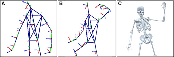
Figure 5 shows preliminary results of two exemplary applications implemented using our presented motion tracking framework. In Fig. 5a-b we interactively changed the pose of the motion captured person by editing the computed rotation angles. Since these parameters correspond to main movements, it is much simpler to apply even significant pose changes compared to working with less intuitive parameterizations. The second example in Fig. 5c shows a skeleton mesh attached to the motion captured data. The normalized coordinate systems greatly reduce the time and work necessary to equip a raw character skeleton with a given mesh. Once aligned, these meshes can generally be used for data from different recording sessions and subjects. Finally the estimated model-parameters allow for the detection and correction of erroneous model poses due to tracking errors in subsequently recorded data, improving the robustness of applications based on real-time tracking and visualization.

In this work we described two processing steps for efficient and automatic normalization and parameterization of optical motion tracking data. This work extends our previously presented pipeline [ HSK05 ], and specifically addresses the requirements of dynamic virtual environments since it does not pose any constraints on the recording setup and needs only a short calibration phase.

During the normalization stage we reliably computed new coordinate systems for the tracked limbs. In contrast to the initial data with a strong dependency on the placement of the marker bodies, they are now consistently aligned with the skeleton structure, yielding a common basis across experiments. Hence, the generated data can be reproduced and compared, with only little time to be invested in the recording preparations, drastically reducing the time needed for motion analysis experiments. Secondly, the coordinate systems are very intuitive to use, and we expect them to simplify tasks such as retargeting.

The data parameterization makes it is possible to define suitable movement axes by simply performing corresponding movements in a short calibration phase. If high accuracy and reproducibility is required, mechanical instruments could be used to restrain the movements of the actor; for most non-medical applications though, especially VR-based applications, the definition of the axes is very simple and does not require such tools.

Based on our experiments we think that the new computation steps could prove useful in many VR-based and optical motion tracking applications to reduce the necessary manual pre-processing steps significantly. In future work we plan to investigate the benefit of our method in a more elaborate and diverse set of VR application settings.

We thank A.R.T. [ Adv ] for kindly providing this project with additional tracking equipment.